AI-Assisted Capture of Missing Physics: PINNs Trained on Wind Tunnel Data on a Single-Board Computer
March 17, 2026
At Re = 3,000,000 — matching experimental conditions — physics-informed neural networks trained on 1959 wind tunnel data capture missing physics that traditional CFD simulations miss entirely. Open-source tools, low-cost hardware, no GPU — driven end-to-end by text commands on Telegram through OpenClaw.
Disclaimer: This work is a technology demonstration. The results have not been independently validated against new experimental campaigns. All experimental data are sourced from publicly available literature. This study should not be used for engineering design decisions without further testing and validation.
The Problem with CFD-Only Training: Missing Physics
Traditional CFD — even advanced RANS and LES — is only as good as the physics it encodes. Turbulence models miss critical real-world phenomena:
- Wing-body interactions: Junction flows produce horseshoe vortices and corner separation that RANS models systematically mispredict.
- Acoustic effects: Trailing-edge noise can interact with boundary layer transition — a coupling absent from most steady simulations.
- Free-stream turbulence and roughness: These influence transition location and separation behavior in ways that require explicit (and often omitted) modeling in CFD.
- Three-dimensional separation: Real separated flows exhibit spanwise structures that two-equation turbulence models cannot resolve.
A PINN trained only on CFD inherits these blind spots. Predictions look smooth but are wrong in the same ways as the source simulation.
The Solution: Train on Real Wind Tunnel Data Instead
In 1959, Abbott and Von Doenhoff published Theory of Wing Sections, compiling decades of NACA wind tunnel data into tables of lift, drag, and pressure distributions. Free for over 60 years.
In 2019, Raissi et al. introduced PINNs — neural networks that learn to satisfy physics equations like Navier-Stokes as part of their training loss.
This project combines both ideas: take the publicly available experimental data from Abbott & Von Doenhoff, combine it with the Navier-Stokes equations as physics constraints, and train neural networks that produce flow fields around a NACA 0014 airfoil. Because the experimental data carries the imprint of all the physics present in the real flow — including wing-body interactions, acoustic effects, tunnel turbulence, and transition — the trained model implicitly encodes phenomena that a CFD-trained model would miss entirely.
Training runs on a ZimaBoard 2 — a low-cost single-board computer drawing just 6 watts.
The Hardware: Low-Cost Edge Computing, No GPU
No GPU. All training on CPU via PyTorch with 4 threads. Total time for all five models: ~74 minutes.
The Data: Publicly Available Wind Tunnel Measurements
All experimental data are sourced from publicly available literature:
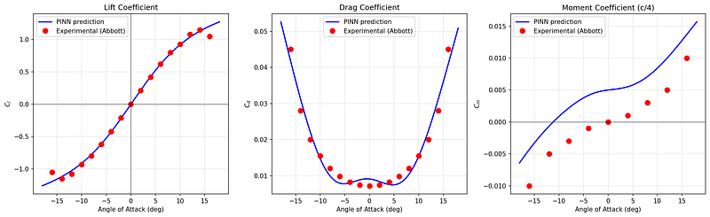
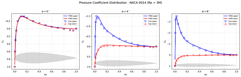
- Abbott & Von Doenhoff (1959): Lift, drag, and moment coefficients at 17 angles of attack from −16° to +16° at Re = 3 million. Pressure distributions at α = 0°, 4°, and 8°.
- NACA Report 460 (1933): Original wind tunnel tests from the Variable Density Tunnel at Langley, including Reynolds number scaling data.
- XFOIL (Drela, MIT): Panel method validation references.
Total: 17 lift, 17 drag, 9 moment, 51 pressure points, 6 Reynolds data points. A small dataset — but with physics constraints, it’s enough.
The Models: Three Neural Networks, Three Tasks
Model 1: Aerodynamic Coefficients (AeroCoeffNet)
A 4-layer fully-connected network (2 → 64 → 64 → 64 → 3) that takes angle of attack (α) and Reynolds number (Re) as inputs and predicts lift coefficient (Cl), drag coefficient (Cd), and moment coefficient (Cm).
The loss function includes not just the data-fitting term, but also physics constraints:
- Symmetry: For a symmetric airfoil, Cl(α) = −Cl(−α) and Cd(α) = Cd(−α).
- Thin airfoil theory: The lift curve slope at small angles should be approximately 2π per radian.
- Drag positivity: Cd must always be positive.
Model 2: Pressure Distributions (CpNet)
A 5-layer network (2 → 80 → 80 → 80 → 80 → 2) that takes chordwise position (x/c) and angle of attack (α) as inputs and predicts the pressure coefficient on the upper and lower surfaces.
Physics constraints include:
- Stagnation condition: Cp → 1 at the leading edge (where the flow comes to rest).
- Kutta condition: Cp → 0 at the trailing edge (smooth flow departure).
- Cp–Cl consistency: The integral of the pressure difference between lower and upper surfaces must equal the lift coefficient.
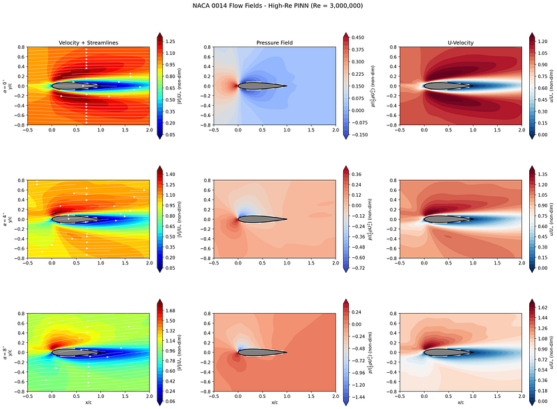
Model 3: Flow Fields (FlowFieldNet)
This is the core physics-informed model. A 6-layer network with 5 hidden layers of 100 neurons each (2 → 100 → 100 → 100 → 100 → 100 → 3) takes spatial coordinates (x, y) as inputs and predicts the velocity components (u, v) and pressure (p). The network operates at Re = 3,000,000, matching the experimental data directly.
The key innovations are the hybrid loss function and curriculum learning:
- Navier-Stokes PDE residual: The network output must satisfy the continuity equation (∇·V = 0) and the momentum equations at 2,000 randomly sampled collocation points per epoch.
- No-slip boundary: Zero velocity on the airfoil surface.
- Experimental data anchoring: Where experimental Cp data are available, the predicted surface pressure is constrained to match.
- Curriculum learning: Viscosity is annealed from Re ≈ 1,000 up to Re = 3,000,000 during training, allowing the network to first learn the large-scale flow structure before resolving the thin boundary layers at the target Reynolds number.
- Near-wall collocation point clustering: Collocation points are concentrated near the airfoil surface to resolve the thin boundary layer at high Reynolds number.
Velocities normalized by U∞; pressures by ½ρU∞². Separate models trained for α = 0°, 4°, 8° — 5,000 epochs each.
From 2D to 3D: Extruding to a Finite Wing
The 2D flow solution at α = 4° is extruded to three dimensions to create a finite wing with chord = 0.2 m and span = 1.0 m. Two physical corrections are applied:
- Elliptic spanwise loading: Following Prandtl’s lifting-line theory, the perturbation velocities are modulated by an elliptic distribution that vanishes at the wing tips and peaks at midspan.
- Lamb-Oseen tip vortices: Counter-rotating vortices at the wing tips create realistic induced velocities and a downwash field.
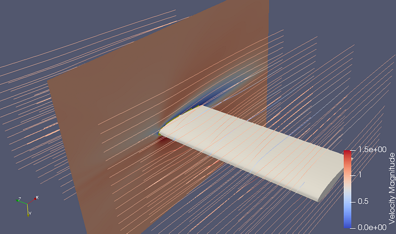
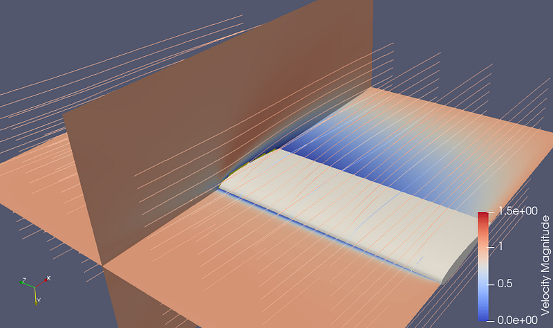
Visualization: ParaView and WebGL
The 3D flow field is exported in two formats:
ParaView files (VTU/VTP): The full 960,000-point volume mesh (with airfoil cells removed), pre-sliced cross-sections, wing surface, and streamlines. These can be opened in ParaView for detailed investigation — color by velocity magnitude, pressure, or any velocity component.

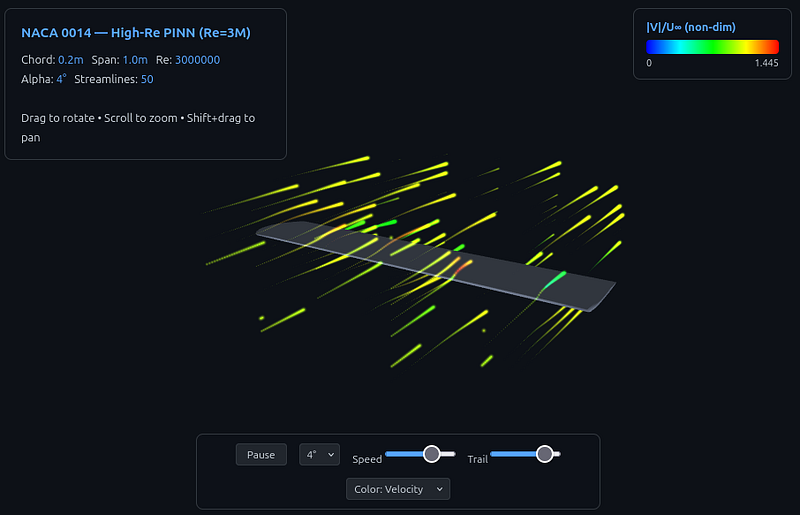
Self-contained HTML animation (CLICK HERE TO ACCESS): A single HTML file with embedded WebGL that runs in any modern browser. Features include:
- 72 animated streamlines traced using 4th-order Runge-Kutta integration
- Toggle between velocity and pressure coloring via a dropdown menu
- Velocity colormap: blue → cyan → green → yellow → red
- Pressure colormap: blue (suction) → white (zero) → red (stagnation)
- Orbit camera, zoom, pan, speed and trail controls
- No external dependencies — everything is self-contained in custom GLSL shaders
- Runs in any WebGL-enabled browser (Firefox, Chrome, Edge) on any OS — no plugins required
Results: How Good Is It?
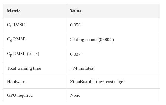
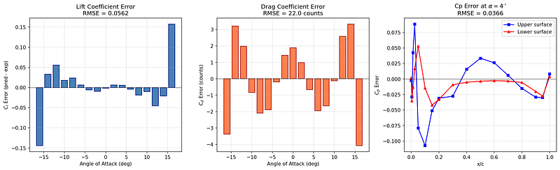
Lift matches well in the linear range (±10°). Largest errors near stall (±16°), expected since the PINN doesn't model separation or transition. Drag polar captures the bucket shape. Pressure distributions agree well across all three angles.
Extended Inference: Seven Angles of Attack
Initial training at 0°, 4°, 8°. Four additional models trained at α = 2°, 6°, 10°, 12° using the same curriculum approach. Each takes ~15 minutes.
Trained Model Capabilities
Once trained, the models serve as rapid-query aerodynamic tools:
- AeroCoeffNet: Query Cl, Cd, Cm at any angle of attack and any Reynolds number — no retraining needed.
- CpNet: Query upper/lower surface pressure distributions at any angle and chord position.
- FlowFieldNet: Full velocity and pressure fields at 7 discrete angles (0° through 12°), each at Re = 3×10⁶.
The LLM Workflow: Code Generation via Natural Language
The entire workflow is driven by natural language instructions through OpenClaw, which provides a Telegram-based interface for sending simulation commands to the ZimaBoard remotely.
OpenClaw supports multiple LLM backends, including:
- Claude Opus 4.6 (Anthropic): Code generation and debugging.
- Z.AI GLM 5: An alternative LLM backend for code generation and iterative development.
Either model can be used interchangeably with OpenClaw to drive the simulation pipeline. From natural language instruction to animated 3D streamlines, the complete turnaround is under one hour on the ZimaBoard 2. No manual coding, no mesh generation, no turbulence model selection required.
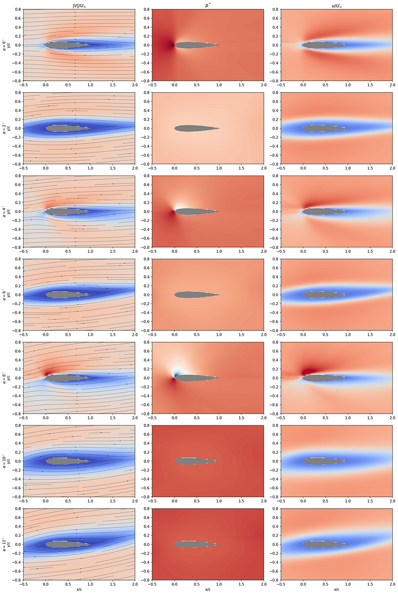
Flow Field Evolution Across Angles
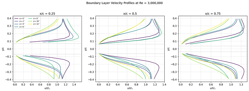
Boundary Layer Profiles
Open Source: No Expensive Licenses Required
A traditional CFD workflow typically depends on proprietary commercial software with annual licensing costs. Add proprietary meshing tools and post-processors, and the software bill alone can exceed the cost of the hardware it runs on.
This entire project uses only open-source software:
- PyTorch — neural network training and automatic differentiation
- NumPy / SciPy — numerical computation, interpolation, integration
- Matplotlib — 2D plotting and figure generation
- PyVista — 3D mesh construction and VTU/VTP export
- ParaView — professional-grade 3D visualization and post-processing
- Linux Mint 22.3 Cinnamon — the operating system
- OpenClaw — the LLM-assisted simulation platform
Complete pipeline — training data to 3D streamlines — with zero licensing cost. Reproducible without buying a single license. Dramatically lowers the barrier to entry for computational aerodynamics.
Limitations and Future Work
Important: This is a technology demonstration. The results have not been validated against independent experiments.
Key limitations include:
- Curriculum sensitivity: The viscosity annealing schedule significantly affects convergence quality. Different annealing rates or starting Reynolds numbers can lead to substantially different results.
- No stall modeling: Flow separation beyond α ≈ 12° is poorly predicted.
- Steady-state only: Unsteady phenomena like vortex shedding are not modeled.
- Simplified 3D: The spanwise extrusion is approximate; real wing tip effects are more complex.
Future work should validate against RANS solutions, optimize the curriculum learning schedule for robust convergence, and incorporate unsteady capability for dynamic stall analysis.
Conclusion
This project demonstrates that meaningful computational aerodynamics at Re = 3,000,000 — matching experimental conditions with no Reynolds number mismatch — can be performed on low-cost edge hardware drawing just 6 watts, with no GPU, in approximately 74 minutes of training time. All training uses publicly available experimental data from the 1930s–1950s combined with physics-informed neural networks and curriculum learning.
More importantly, it demonstrates a fundamental shift in philosophy: instead of trying to model every physical mechanism from first principles (and inevitably missing some), we can ground our neural networks in experimental measurements that already contain all the physics. By training at Re = 3,000,000 — the same Reynolds number as the wind tunnel experiments — there is no Reynolds number gap between the model and the data. Wing-body interactions, acoustic effects, transition, turbulence — they are all encoded in the wind tunnel data, waiting to be learned. Traditional CFD will remain essential for detailed design and diagnostics, but for applications where fidelity to real-world performance matters most, experimental-data-informed PINNs offer a compelling alternative.
The era where good data + solid physics + low-cost computing + the right tools is all you need is just beginning.