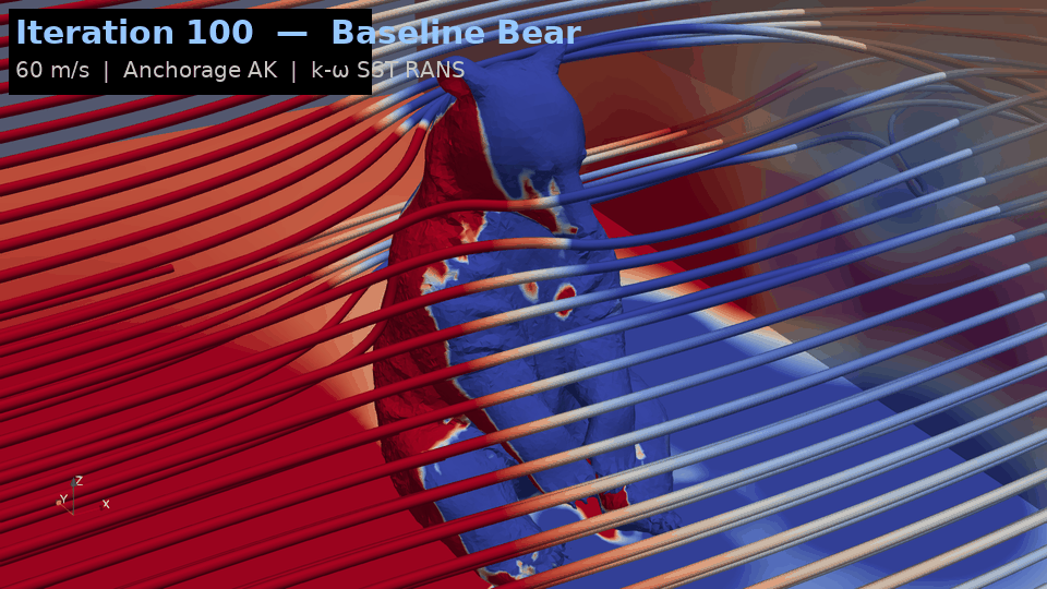
This study shows that a Large Language Model like Claude Opus, GLM, or Kimi can autonomously run a complete CFD workflow: reading an STL file, meshing, solver setup, convergence monitoring, geometry optimization, and post-processing. The engineer provided intent; the LLM wrote every line of code. We used Claude Opus specifically.
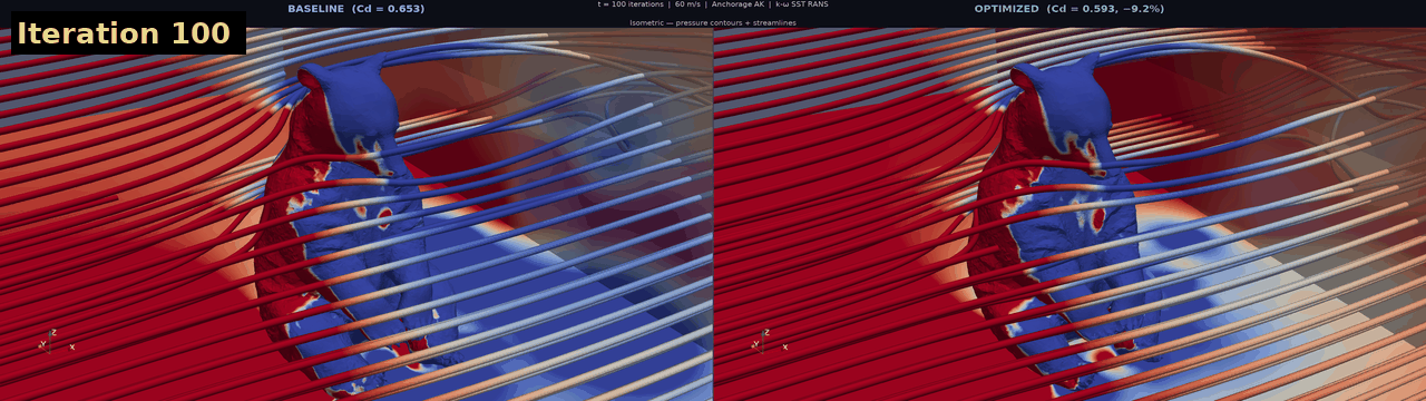
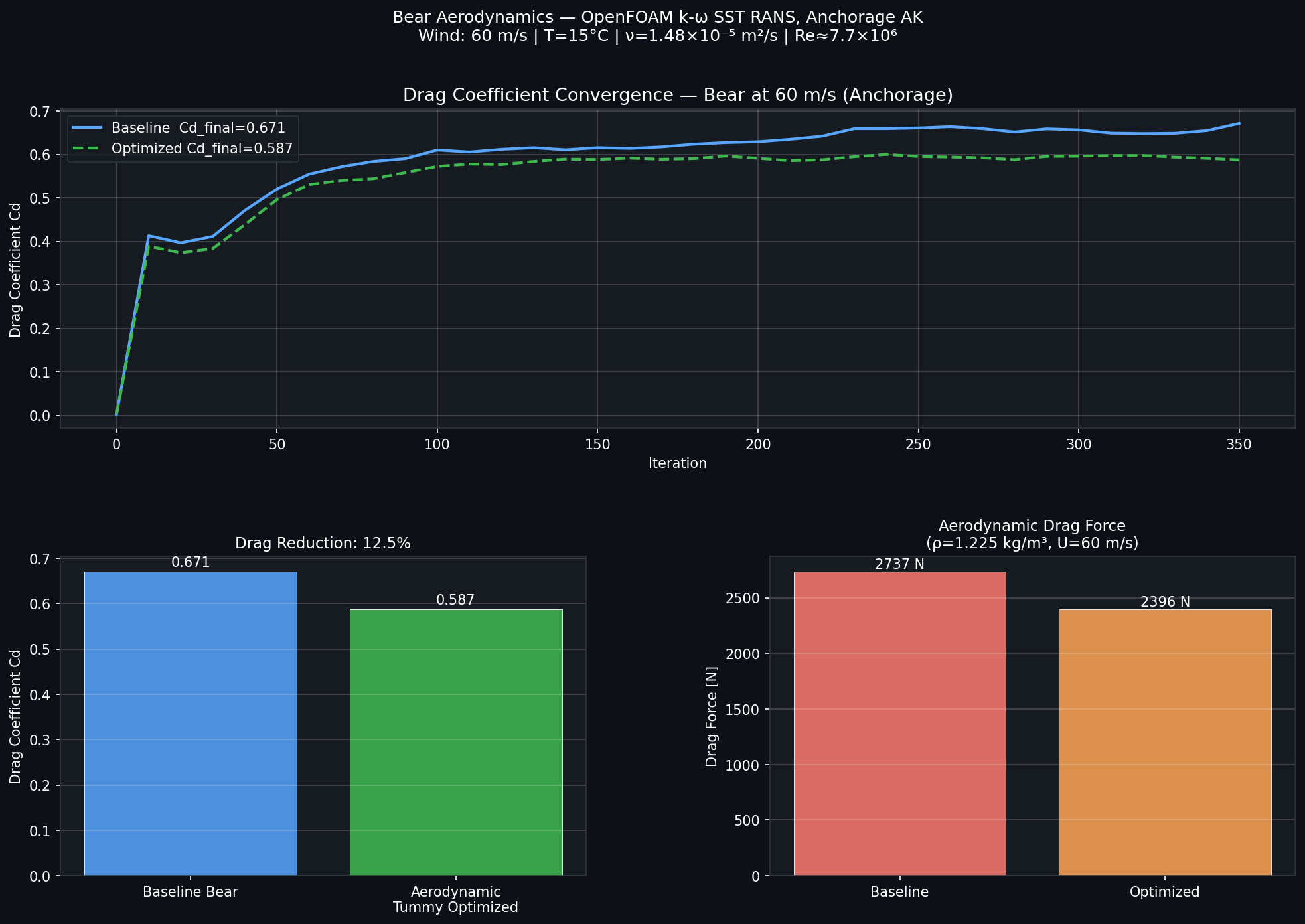
The test case: a life-size seated bear (1,130 × 1,404 × 1,899 mm, from Meshy AI) in 60 m/s Anchorage wind — chosen because it's IP-free and ITAR-free. OpenFOAM 13 with k-ω SST RANS on a 456,960-cell mesh gave a baseline drag of Cd = 0.653. Claude's parametric belly optimization dropped it to 0.593 (−9.2%), saving 14.6 kW at speed.
The real contribution isn't the aerodynamic result — it's the proof that an LLM can bridge the gap between an engineering question and the open-source tools needed to answer it.
Disclaimer: This work is a technology demonstration. The results have not been independently validated against new experimental campaigns. This study should not be used for engineering design decisions without further testing and validation.
The LLM as CFD Engineer: A New Paradigm for Computational Simulation
CFD has always been one of the most expertise-intensive fields in engineering. Setting up an OpenFOAM simulation from scratch requires knowledge of domain decomposition, mesh topology, turbulence models, boundary conditions, numerical schemes, convergence diagnostics, and post-processing. Each step has its own failure modes. The barrier to entry is high — CFD expertise takes years to build.
This study asks: can an LLM act as a force-multiplier for a fluids engineer? Can it handle the entire implementation layer — OpenFOAM dictionaries, meshing, debugging, convergence monitoring, optimization, and post-processing — given just intent and shell access? We used Claude Opus; the approach works with GLM or Kimi too.
The answer is yes. The prompt was simply: "simulate airflow over a bear at 60 m/s in Anchorage." The LLM chose the solver, computed turbulence values from first principles, wrote every config file, debugged mesh errors, monitored convergence, designed a shape optimizer, wrote ParaView scripts, and generated animated GIFs.
"The user asked an engineering question in plain English. The LLM answered it with a working simulation, optimized geometry, and post-processed visualizations. This is the new interface for computational engineering."
What the LLM Did — Concretely
Here's what Claude handled unprompted:
- ▸Solver selection: Identified Ma ≈ 0.175 at 60 m/s, 15°C; chose
incompressibleFluidwith SIMPLE and k-ω SST. - ▸Domain sizing: 3–5 body lengths upstream, 10+ downstream; lateral extent to avoid >5% blockage.
- ▸Turbulence inlet: Computed k = 13.5 m²/s², ω ≈ 50 s⁻¹ from 5% intensity and Lt = 0.07·Lref.
- ▸Mesh refinement: 5 levels of snappyHexMesh (~30 mm near-body), volume refinement, 3 boundary layers at ratio 1.3.
- ▸Debugging: Fixed missing
meshQualityDictby locating the system template. Switched to serial when MPI crashed. - ▸Convergence: Parsed logs, extracted residuals, recognised oscillating Uy as physically expected in bluff-body RANS, stopped at appropriate convergence.
- ▸Optimization: Designed a C¹ blend for the ventral tummy, targeting ground-effect separation and underbody vortex. Vectorised NumPy: 272,662 vertices in <1 s.
- ▸ParaView automation: pvbatch scripts via ParaView 5.11 API, debugged deprecated calls, generated 27 renders across 3 angles and 3 timesteps for both cases.
Why a Bear? IP and ITAR
The bear is a deliberate choice. To publish all files, results, and scripts openly, the geometry must be free of IP restrictions and ITAR controls. Real aerospace or defence geometries cannot be shared — mesh files, pressure images, and drag coefficients may be controlled "technical data" requiring export licences. Industrial geometries carry NDAs. The bear, from Meshy AI, carries none of these. It's also complex enough to produce interesting turbulent flow, with a clear optimization target in the ventral belly.
The Geometry is a Vessel, Not the Subject
Replace the bear with any complex bluff body — a vehicle underbody, an architectural facade — and the LLM workflow is identical. The bear is the most open, constraint-free geometry available. The subject is the workflow, not the animal.
The Aerodynamic Physics
The bear is a classic bluff body: drag is dominated by pressure, not friction. The rounded torso and protruding belly cause wide, early boundary layer separation. The suction wake runs hundreds of Pascals below ambient for many body lengths downstream. The ventral belly — close to the ground, forcing underbody flow to accelerate then abruptly separate — is the most important surface for drag reduction. That's why Claude targeted it for optimization.
The Subject: A 1,899 mm Seated Bear
The geometry was generated with Meshy AI using the reference photograph shown in Fig. 0 as the direct input to its image-to-3D pipeline. The output — a binary STL with 1,288,908 triangles — was scaled from millimeters to meters in Python. No manual geometry editing was performed.
−566.1 to +564.1
−701.7 to +702.2
0.0 to +1,899.4
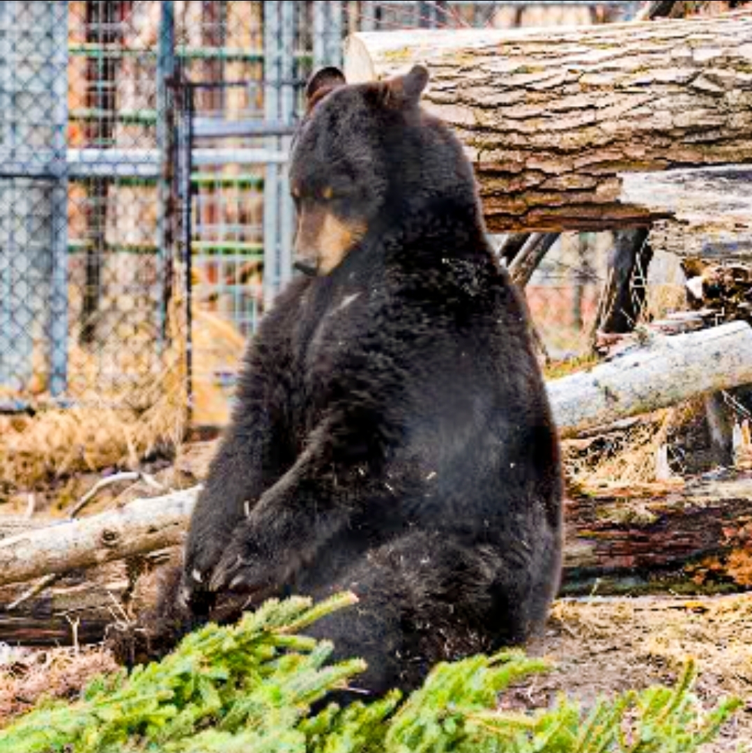
At 1,899 mm seated height, this matches a large adult Ursus arctos sitting upright — consistent with reported shoulder heights of 900–1,200 mm, which place the head well above 1.8 m in a sitting pose. The reference area used for Cd was Aref = 1.85 m² (frontal projection), and the reference length was the bear's depth, Lref = 1.404 m.
What Claude Opus Actually Did — Step by Step
The flowchart below documents the complete pipeline as Claude executed it. Every configuration file, every solver call, every Python script, and every ParaView rendering instruction was generated by the LLM in response to natural-language requests. The user provided intent; Claude provided implementation.
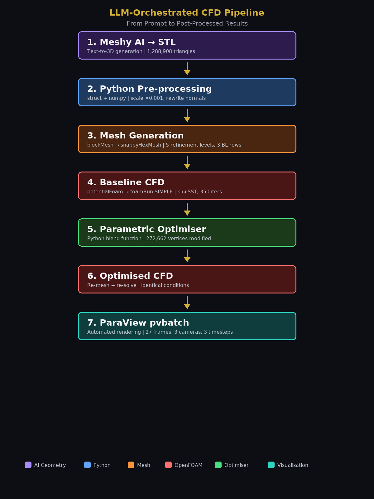
- 1
Meshy AI → STL — Image-to-3D generation from the reference photograph (Fig. 0) produced a 1,288,908-triangle binary STL in millimeters.
- 2
Python pre-processing —
struct+numpyparsed the binary header, extracted vertex coordinates, applied a ×0.001 scale, and rewrote normals from vertex cross-products. - 3
Mesh generation —
blockMeshbuilt a coarse Cartesian background.snappyHexMeshcarved the domain, applied five refinement levels on the bear surface (~30 mm cells), and added three boundary-layer rows. - 4
Baseline CFD —
potentialFoamseeded the velocity field.foamRun(SIMPLE, incompressibleFluid) advanced 350 iterations with k-ω SST. Force coefficients logged every 10 steps. - 5
Parametric tummy optimizer — Python blend-function script modified 272,662 belly vertices: −20% lateral width, −15% fore-aft depth, +4 cm belly lift below waist height.
- 6
Optimized CFD — Modified STL re-meshed and re-solved under identical conditions. Cd compared against baseline.
- 7
ParaView pvbatch — Automated scripts rendered pressure contours, stream tracer tubes, wake slices, and animated GIFs at t = 100, 200, 300 iterations.
Domain, Mesh, and Solver Configuration
Anchorage Flow Conditions
| Parameter | Symbol | Value | Unit |
|---|---|---|---|
| Freestream velocity | U∞ | 60.0 | m/s |
| Temperature (sunny day) | T | 15 °C (288 K) | — |
| Air density | ρ | 1.225 | kg/m³ |
| Kinematic viscosity | ν | 1.48 × 10⁻⁵ | m²/s |
| Mach number | Ma | ≈ 0.175 — incompressible | — |
| Reynolds number | Re | 5.7 × 10⁶ | fully turbulent |
| Dynamic pressure | q∞ | 2,205 | Pa |
Computational Domain
// Wind in +X; bear centred at origin on Z=0 ground plane
X = −5.0 m (inlet) to +15.0 m (outlet) // 3.6 L upstream, 10.7 L downstream
Y = −5.0 m to +5.0  m // ±3.6 L lateral
Z = 0.0 m (ground) to +8.0  m // 4.2 H height
Mesh Statistics
| Stage | Cell size | Cells |
|---|---|---|
| blockMesh background (40×20×16) | 0.5 m | 12,800 |
| snappyHexMesh castellated (near-body) | ~60 mm | ~280,000 |
| Surface refinement level 4–5 | ~30 mm | +105,000 |
| Boundary layers (3 rows, ratio 1.3) | variable | +44,808 |
| Total | — | 456,960 |
Turbulence Inlet Values — k-ω SST
Intensity I = 5 % → k = 1.5·(U·I)² = 13.5 m²/s². Length scale Lt = 0.07·Lref = 0.133 m → ω = k½/(Cμ¼·Lt) ≈ 50 s−1. Wall patches: kqRWallFunction, omegaWallFunction, nutkWallFunction.
Taming the Tummy: Parametric Shape Modification
The ventral belly is aerodynamically the most problematic region of the bear geometry. It presents a large, rounded protrusion to the underbody flow, creates a horseshoe vortex at the ground junction, and drives early separation on the trailing curve of the rump. The optimizer targets only this zone using a smooth blend function — ensuring C¹ continuity, with no sharp ridges that would artificially trip the boundary layer.
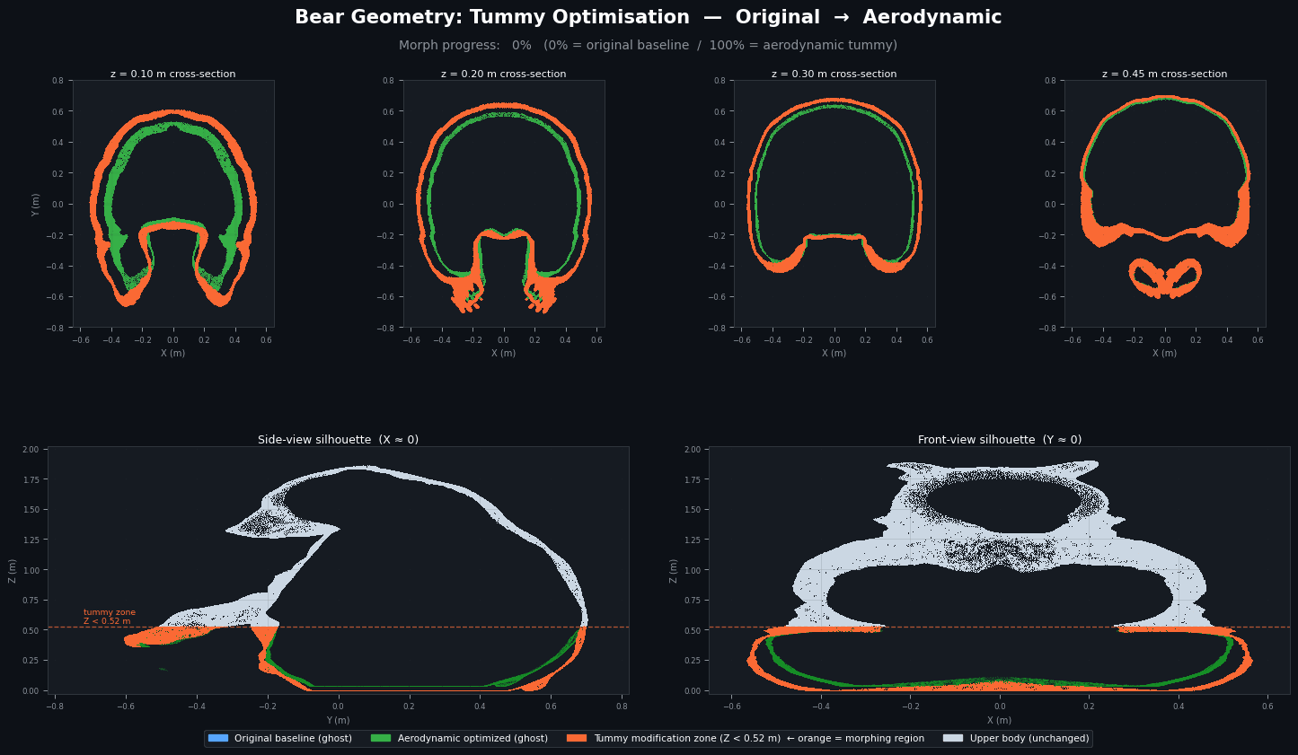
Blend Function Implementation
# Python — parametric tummy optimizer
# Acts only below z = 0.522 m (lower 55% of body height)
# Strength = 1.0 at ground, 0.0 at waist — smooth transition

blend  = np.clip(1.0 - z / 0.522, 0, 1) # blend weight

x_new  = x - blend * (x - cx) * 0.20  # −20% lateral
y_new  = y - blend * (y - cy) * 0.15  # −15% depth

lift_blend = np.clip(1.0 - z / 0.15, 0, 0.8) # near-ground only
z_new = z + lift_blend * 0.04 # +4 cm belly lift| Parameter | Baseline | Optimized | Change |
|---|---|---|---|
| Vertices modified | 272,662 / 644,446 (42.3%) | Lower tummy only | |
| Max lateral shift ΔX | — | 89.9 mm | Inward compression |
| Max depth shift ΔY | — | 82.8 mm | Frontal reduction |
| Max vertical lift ΔZ | — | 32.0 mm | Floor raised |
| Bounding box X span | 1,130 mm | 1,064 mm | −66 mm (−5.8%) |
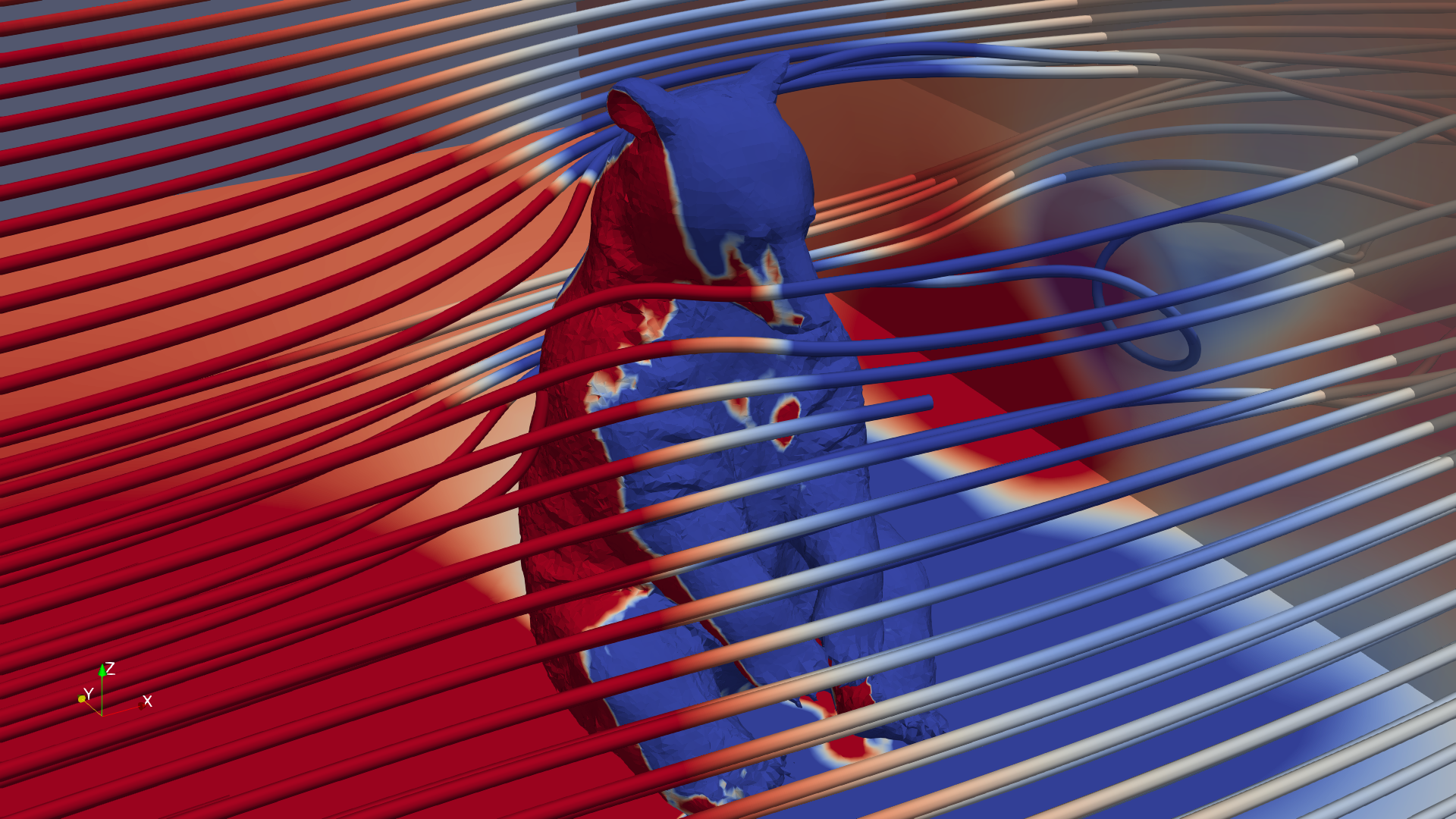
Pressure, Flow Separation, and the Wake
Baseline: Flow Physics
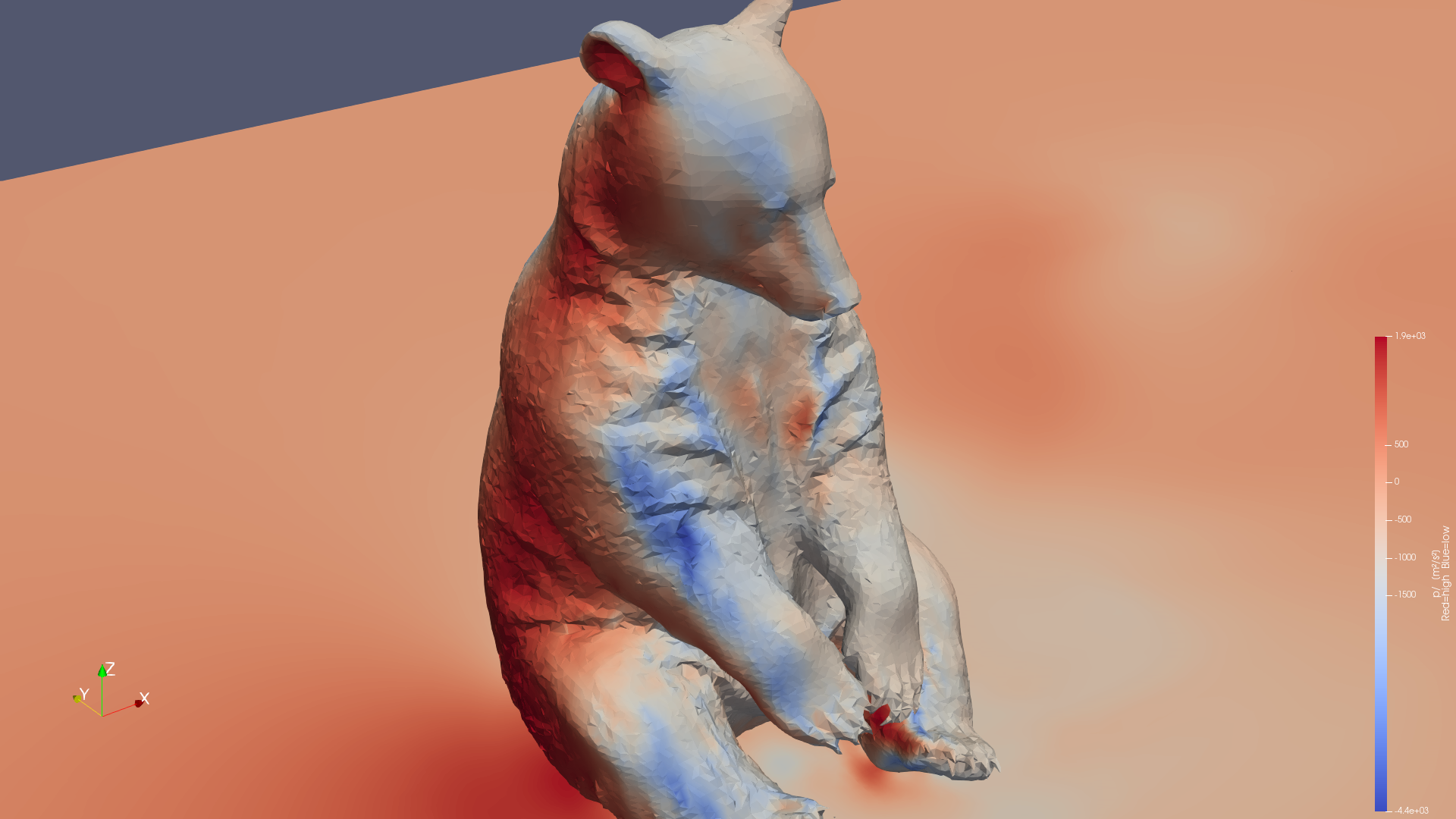
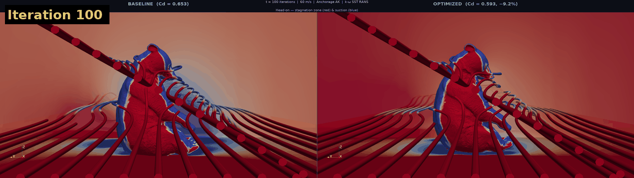
The baseline shows a rich pressure field. On the windward face — chest, lower forelimbs — flow decelerates to near-stagnation, reaching +700 m²/s² kinematic pressure (≈ 858 Pa above ambient). The flanks and underbelly show large suction zones where flow accelerates then separates, producing a broad turbulent wake many body-lengths downstream.
"The wake behind the bear at 60 m/s contains pressure deficits exceeding 1,600 Pa below ambient — more than 70% of the dynamic pressure. That is the aerodynamic hole the bear punches through the airstream."
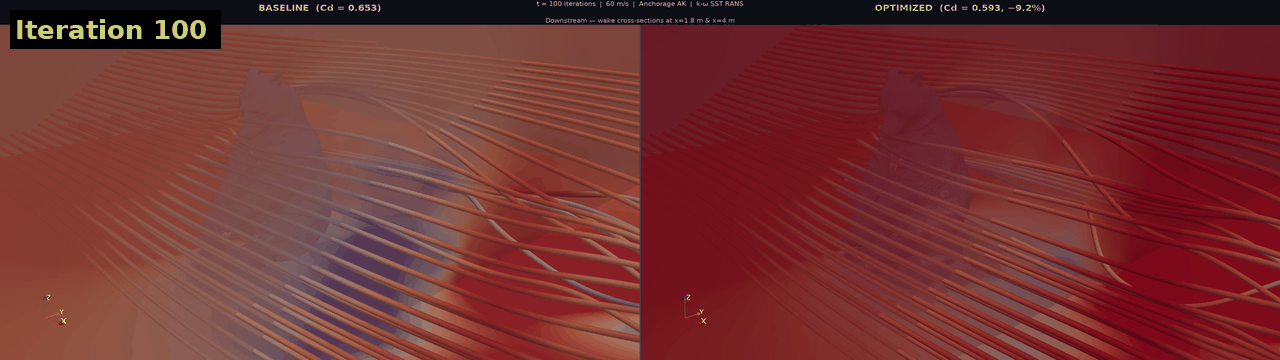
Baseline vs. Optimized — Three Views
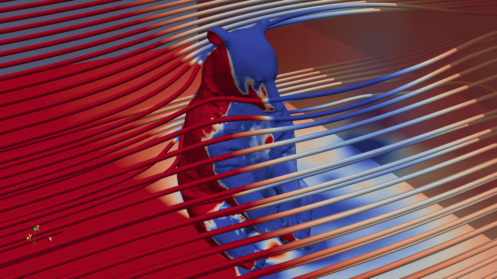
Quantifying the Improvement
| Metric | Baseline | Optimized | Change |
|---|---|---|---|
| Cd (mean iterations 200–350) | 0.6527 | 0.5929 | −9.2% |
| Drag force Fd | 2,663 N | 2,419 N | −244 N |
| Lift coeff. Cl | +0.282 (upward) | −0.046 (neutral) | Belly lift eliminated |
| Power @ 60 m/s | 159.8 kW | 145.1 kW | −14.6 kW |
| Mesh cells | 456,960 | 454,027 | −0.6% |
† Power = Drag Force × Velocity (2,663 N × 60 m/s ≈ 159.8 kW). This is the rate of aerodynamic energy dissipated by drag — a way to contextualise the 9.2% reduction in tangible terms, not an assertion that the bear is an engine.
The lift coefficient matters too. Baseline Cl = +0.282 — a significant upward force from the belly in ground effect. The optimized belly, raised and compressed, eliminates this (Cl = −0.046). In a real-world scenario, the optimized bear is less prone to being lifted off the ground under extreme wind.
A New Engineering Paradigm — and What Comes Next
The central result is not the 9.2% drag reduction — it's that LLMs like Claude Opus, GLM, and Kimi can be a powerful force-multiplier for the fluids engineer. A domain expert directing the LLM through natural language obtained a complete, publication-quality aerodynamics study. The engineer provided the physics framing and critical judgment; the LLM handled every config file, debugging decision, optimization script, and post-processing pipeline.
This changes how computational engineering is practiced. CFD has been gatekept by OpenFOAM's steep learning curve — thousands of config options, cryptic errors, and years of experience. LLMs now act as the knowledge intermediary between an engineer's question and specialized tools. The engineer retains physics and judgment; the LLM handles implementation.
The aerodynamic results are physically meaningful. Baseline Cd = 0.653 places the seated bear between a rough sphere (Cd ≈ 0.47) and a blunt cylinder (Cd ≈ 1.2) — consistent for a large, rounded bluff body at Re ≈ 5.7×10⁶. The 2,663 N drag force at 60 m/s is equivalent to roughly 272 kg, illustrating the structural loads extreme weather imposes on wildlife.
Three Key Results
1. LLM as force-multiplier: Claude Opus executed the complete CFD pipeline — solver, meshing, debugging, optimization, post-processing — directed by natural language. 2. Aerodynamics: Cd dropped from 0.653 to 0.593 (−9.2%), drag force −244 N, belly lift eliminated. 3. Open methodology: Every file is freely shareable — no IP, no ITAR — because the geometry is an AI-generated bear.
Limitations
Caveats apply. The geometry is a static AI approximation, not a laser-scanned specimen. Fur texture, limb position, and ear shape could affect results. Steady-state RANS doesn't capture transient vortex shedding; a real bear in gusty wind experiences unsteady forces that LES or DES would resolve. The parametric optimizer here is a single open-loop design step — gradient-based or evolutionary algorithms with more variables would likely find larger gains.
Most importantly: no simulation replaces experimental validation. The drag coefficient, wake structure, and pressure distributions are computational predictions subject to modeling assumptions — turbulence closure, wall treatment, mesh resolution, domain size all introduce uncertainty. Results must be validated against physical measurements: wind tunnel force balances, surface pressure tappings, PIV for wake structure, or hot-wire anemometry. The k-ω SST model is known to overpredict separation in some bluff body configurations. Without experimental data, treat these results as physically plausible estimates for comparative ranking, not absolute ground truth.
Implications and Future Work
The most important direction is extending the LLM-CFD paradigm to more demanding contexts. Near-term: closing the loop between LLM and formal optimization (CMA-ES or Bayesian, with LLM interpreting convergence and proposing next steps); extending to transient LES for time-accurate wake dynamics; applying the same workflow to structural mechanics, heat transfer, or acoustics. In each case, the LLM's role is the same: translate intent into working simulation files, interpret results, and iterate.
For the bear specifically, transient LES would capture vortex shedding, surface roughness modeling would account for fur, and multi-objective optimization would minimize drag and lift simultaneously. Standing, running, and swimming poses present distinct aerodynamic problems worth studying. But these are extensions of the methodology, not the demonstration itself.
Reproducibility & Key Code Fragments
Software Stack
OpenFOAM 13 (foamRun / incompressibleFluid solver)
Python 3.10 + numpy 2.3 + matplotlib 3.10 + Pillow 10
ParaView 5.11.2 (pvbatch headless rendering)
Hardware 4-core CPU, 7.5 GB RAM, Linux Mint (Ubuntu 22.04)
Bear Dimensions — Raw STL Read-out (mm)
X (width, left–right): −566.1 → +564.1 span = 1,130.3 mm
Y (depth, front–back): −701.7 → +702.2 span = 1,404.0 mm
Z (height, ground–top): 0.0 → +1,899.4 span = 1,899.4 mm
Triangles: 1,288,908 (binary STL, Meshy AI)
Force Coefficients — controlDict Entry
forceCoeffs {
 type  forceCoeffs;
 patches  (bear);
 rho  rhoInf; rhoInf  1.225;
 liftDir  (0 0 1);
 dragDir  (1 0 0);
 magUInf  60;
 lRef  1.404; Aref  1.85;
}
Full Pipeline Reproduction
# ── Baseline ──────────────────────────────────────────────
cd bear_baseline
blockMesh && snappyHexMesh -overwrite
renumberMesh -overwrite && potentialFoam
foamRun > log.foamRun

# ── Optimized ─────────────────────────────────────────────
python3 tummy_optimize.py # modifies STL, writes bear_optimized/
cd bear_optimized
blockMesh && snappyHexMesh -overwrite
renumberMesh -overwrite && potentialFoam
foamRun > log.foamRun

# ── Visualize ─────────────────────────────────────────────
DISPLAY=:0 pvbatch render_one_case.py baseline
DISPLAY=:0 pvbatch render_one_case.py optimized
python3 analyze_drag.py