The brief. One detailed request to an AI agent: design a modern narrow-body airliner as parametric CAD, fly it through full-scale CFD in OpenFOAM, analyse the whole structure in CalculiX, couple the wing’s fluid and structure through preCICE, and write the lot up in LaTeX.
The machine. All of it ran on a ZimaBoard 2, a single-board computer with a quad-core Intel N150 and 8 GB of memory. The CAD remains a live, editable SolidCraft document, and every analysis tool is free and open source, the same codes that companies and research laboratories run at scale.
The outcome. A 68-feature parametric aircraft, a two-million-cell transonic flow solution, a 15,300-element structural model loaded by that flow at 1 g and 2.5 g, a wing coupling that completed one direction of its exchange but not the other, and a 1:500 model ready to print for a desktop wind tunnel. Every artefact was produced by an agent driving real tools, not by a person at a screen.
Disclaimer: This is a technology demonstration. The half-model mesh is a first-pass snappyHexMesh grid with no formal grid-convergence study, and the shell idealization and truncated coupling carry their own caveats. None of it has been validated against wind-tunnel or flight data. No simulation replaces experimental validation. The results are shown for demonstration purposes only and must not be used for engineering design decisions.
01 The pipeline
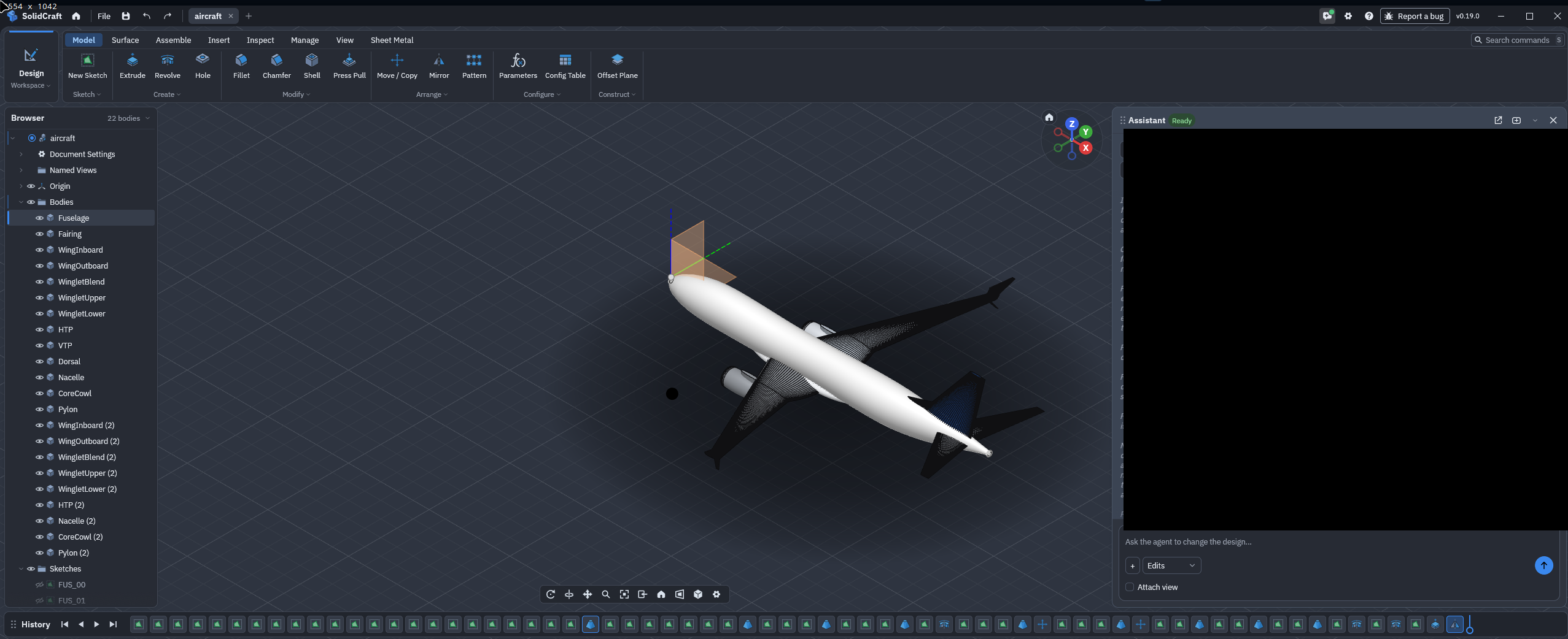
Most “AI designs a product” demonstrations end with a script and a static mesh. This one is different in one crucial respect: the agent lives inside the CAD system. SolidCraft exposes its modelling kernel as commands an LLM can call, sketches, lofts, mirrors and named parameters, so the aircraft is authored the way an engineer would author it, and everything downstream comes straight from the solvers.
02 Geometry
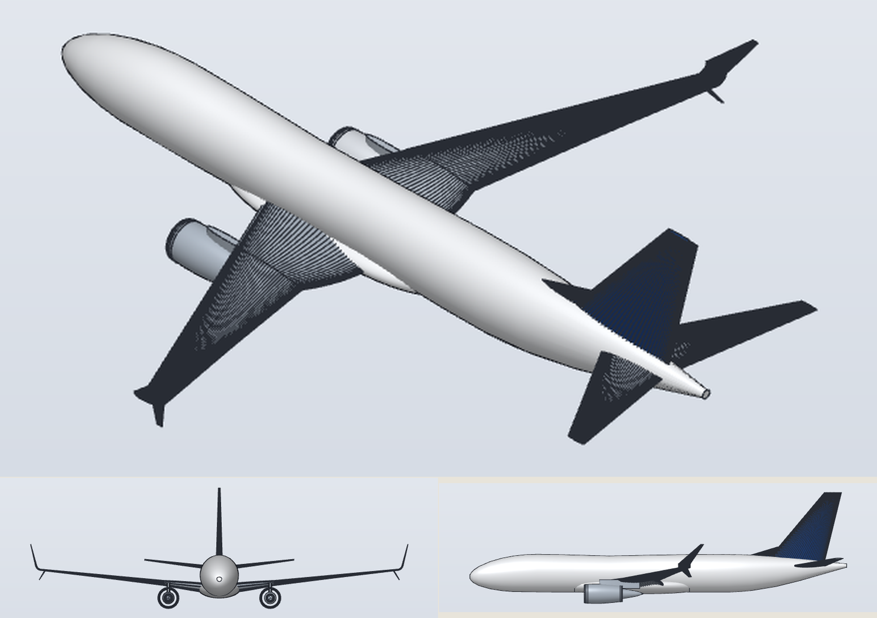
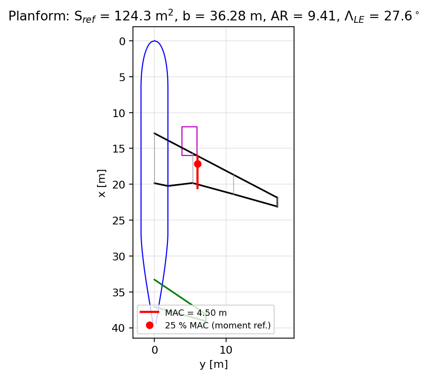
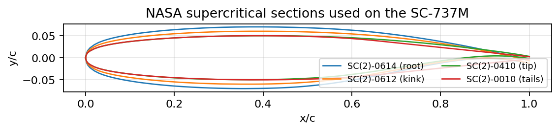
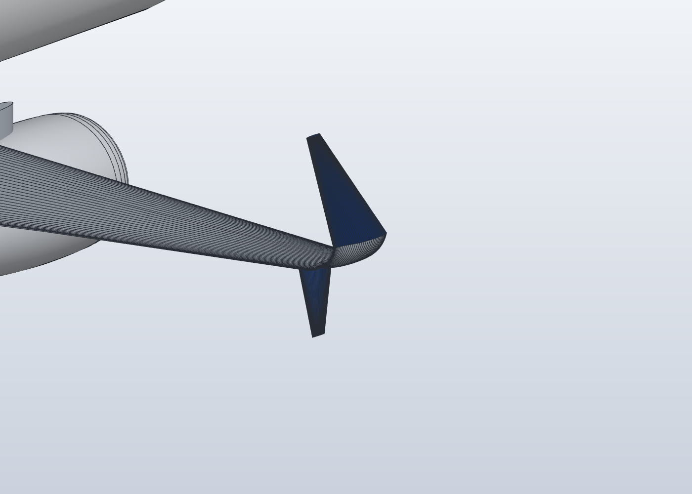
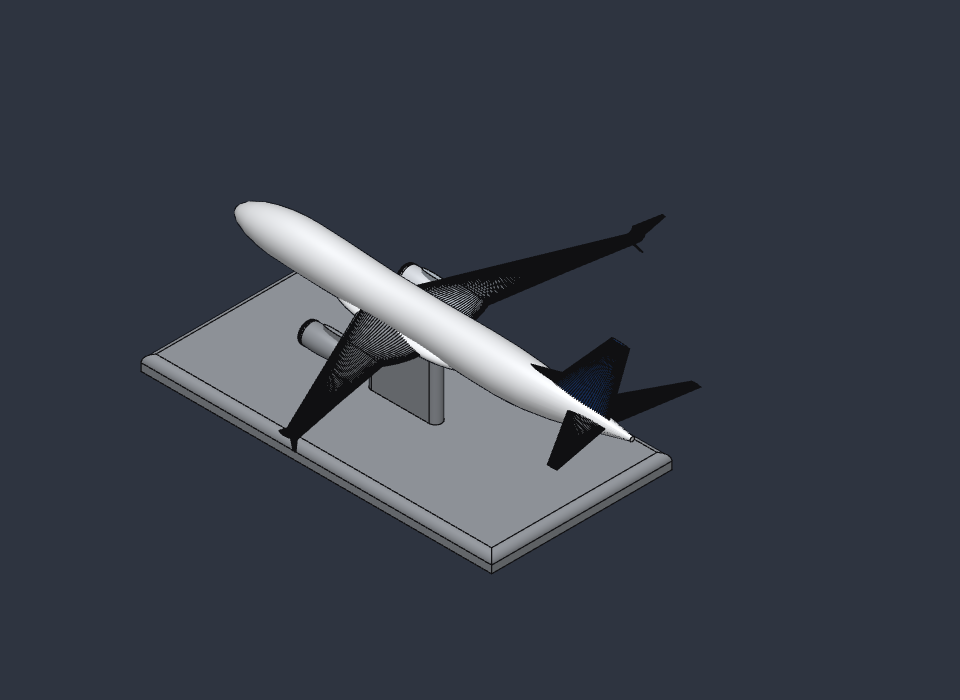
The airframe takes shape the way a seasoned parametric modeller would build it. The fuselage is lofted through 23 sections to an extended tail cone. The wing uses NASA’s SC(2) supercritical sections, swept at 27.6° with 6° of dihedral and a twist toward the tip, and finishes in a split-scimitar winglet with a small ventral feather. High-bypass nacelles hang on pylons, and the tails, dorsal fin and wing–body fairing complete the shape before a single mirror operation produces the other half.
Every feature sits in the design timeline with named parameters. Span, sweep or engine position can be changed later and the aircraft rebuilds itself; the file remains real CAD, not a frozen mesh.
03 Into the airflow
For the flow solution, OpenFOAM’s snappyHexMesh wrapped every component into a single watertight domain of about two million cells for half the aircraft, with thin layers hugging the skin. The aircraft was then flown at a typical cruise point, Mach 0.785 at 35,000 ft with 2° of incidence, using a steady compressible RANS solver with the k–ω SST turbulence model.
The tail of the run settled around a lift coefficient of 0.37 and a drag coefficient of 0.093, with a buffet-like oscillation that the report deliberately keeps rather than averaging away. The animations also exposed a weakness worth stating plainly: about 17 % of the surface sits on the solver’s lower pressure limit, so the aft flow and the integrated coefficients should be treated as unconverged until the case is rerun without that clamp.
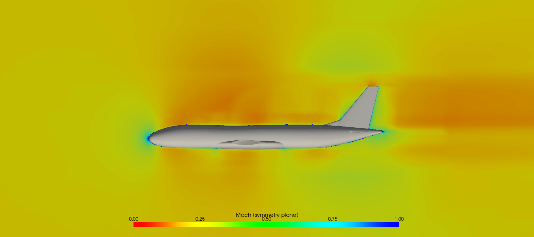
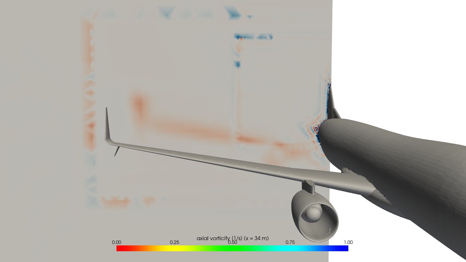
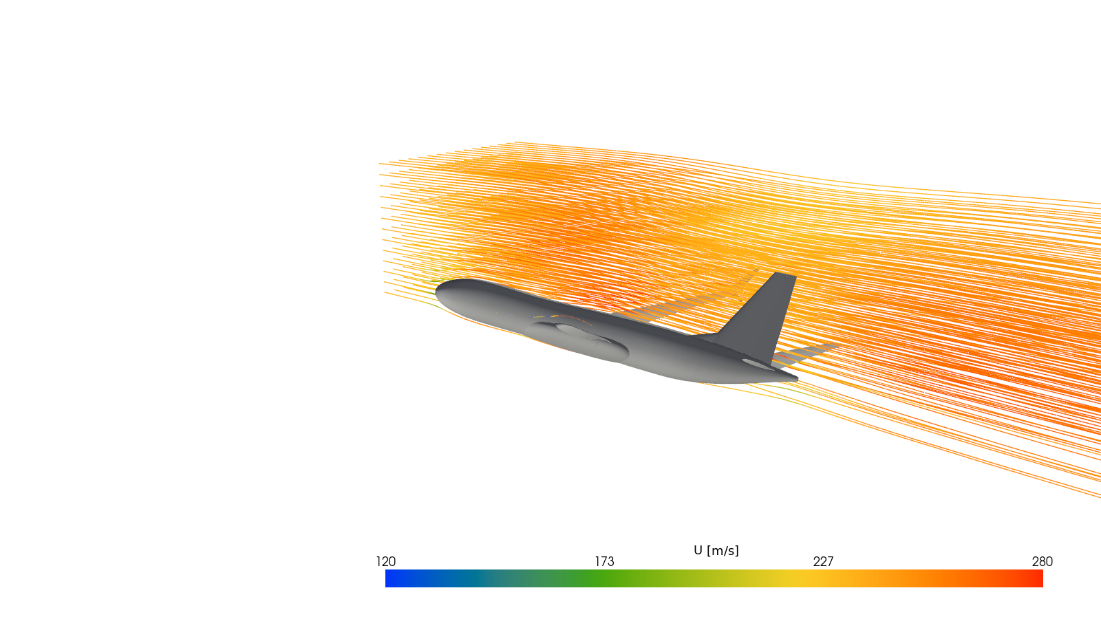
Set in motion, the same solution reveals its transonic character. Particles ride the computed streamlines at their true relative speeds, so one that accelerates over the wing really does pull ahead of its neighbours. Halfway out along the wing, the flow over the upper surface goes supersonic, peaking near Mach 1.07, and slows again well before the trailing edge: exactly the behaviour a supercritical section is shaped to produce.
04 The whole aircraft under load
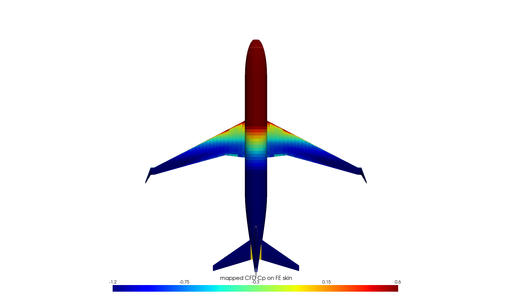
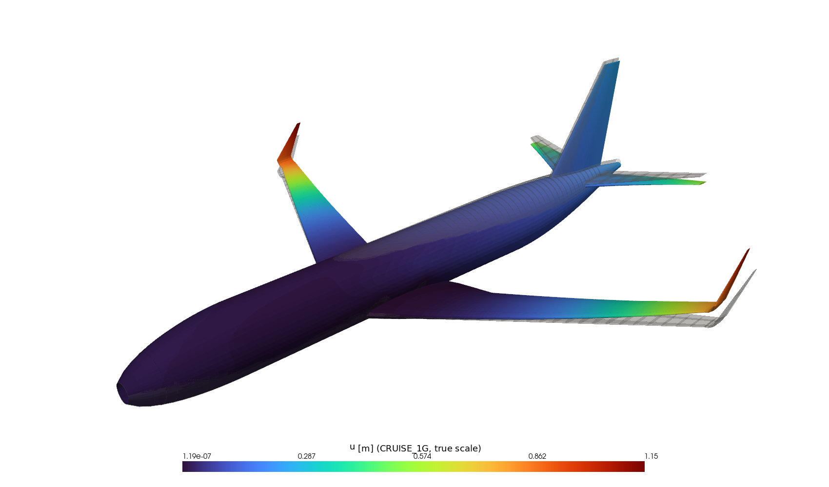
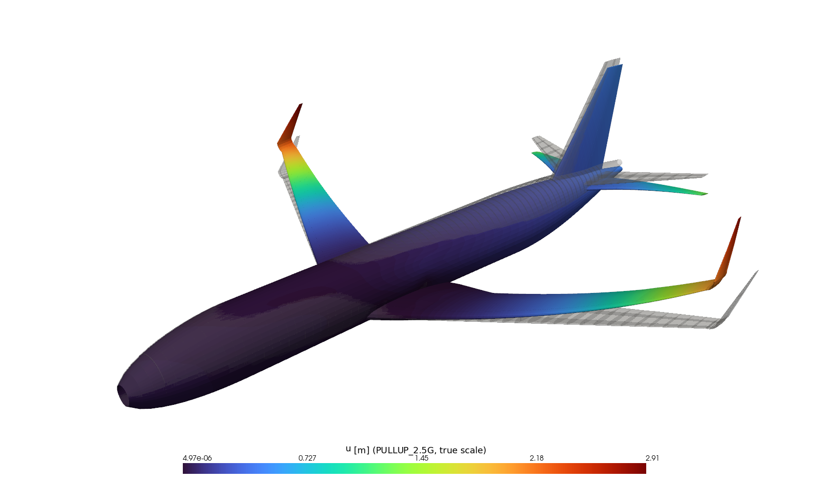
A generator script turned the same geometry into a classic semi-monocoque structure of about 15,300 shell elements: fuselage skins, frames and pressure bulkheads, wing skins, spars and ribs, the tails and the winglets, in aluminium alloys 2024 and 7075. Seventy tonnes of mass, engines and fuel included, were distributed through it. The CFD pressure field was mapped onto the skins and re-trimmed, cabin pressure and inertia were added, and CalculiX solved two cases: steady 1 g cruise and a 2.5 g pull-up.
05 When the wing talks back
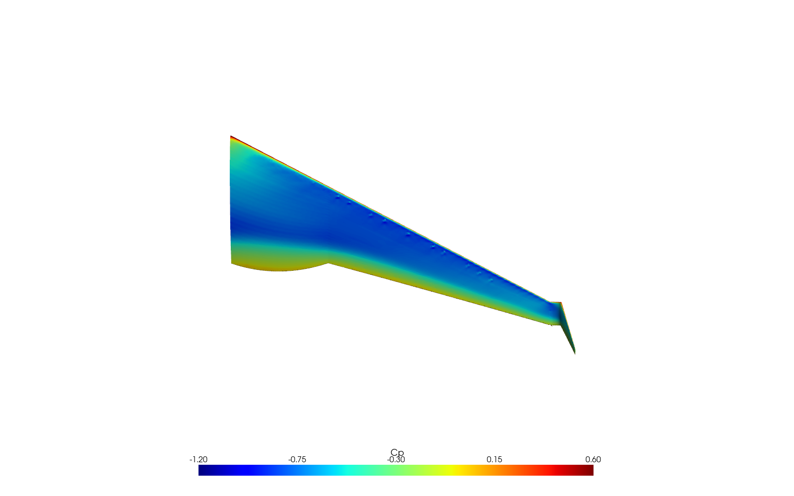
The most ambitious step coupled the flow and the wing structure directly through preCICE. OpenFOAM computed the aerodynamic forces on the wing surface; those forces were transferred, with their total conserved at 410 kN of lift on the half-wing, onto the nodes of a 2,108-node shell model; and CalculiX bent the wing through 40 nonlinear load steps. The result, a winglet-tip deflection of about 0.88 m and a peak stress of 165 MPa, sits comfortably alongside the 1.05 m predicted by the whole-aircraft model at 1 g.
The return journey, moving the fluid mesh to follow the deflected wing, is where this run stopped, and the report says so rather than papering over it.
06 Off the screen: a model for the wind tunnel
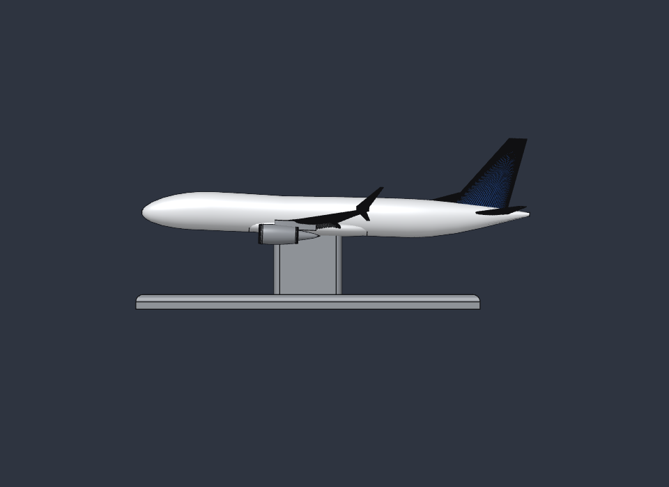
Because the CAD is a living parametric document, the same file also produced something you can hold: a print package for a desktop smoke tunnel. The tunnel’s test section measures just 107 × 92 × 50 mm, far too small for a model at its nominal scale, so the aircraft was printed at 1:500, measuring 78.9 by 72.6 mm. A slender streamlined strut and base plate, both driven by a single scale parameter in the CAD, hold it nose into the flow at the same 2° cruise attitude used in the CFD.
It is a tool for pictures rather than numbers. At such a small size the Reynolds number is a few hundred against tens of millions in flight, so what the smoke reveals is how the flow attaches, where the tip vortex forms and how the wake trails away.
07 What this actually means
The striking number here is not a coefficient. It is the time between intent and evidence: a parametric airframe in minutes, industrial solvers in hours, and a formatted report at the end, all on a computer the size of a paperback. These are credible engineering analyses rather than certification-grade validation, and transonic buffet, structural simplification and an unfinished coupling all leave their fingerprints, which the report keeps in plain view.
The lesson of the simulation-on-simulation essay applies here too. The value of the agent is not a pretty picture. It is the discipline to run the real tool and show the real number, crash logs included.
Tools & references
- OpenFOAM (OpenFOAM Foundation, v13): snappyHexMesh + compressible SIMPLE solver; k–ω SST closure after Menter, AIAA Journal 32(8), 1994.
- CalculiX (Guido Dhondt): nonlinear static solver; ccx_preCICE adapter.
- preCICE: partitioned fluid–structure coupling; Chourdakis et al., Open Research Europe 2:51, 2022.
- NASA SC(2) supercritical airfoil family: Harris, C.D., NASA Supercritical Airfoils, NASA TP-2969, 1990.
- LaTeX / TeX Live: report build; PyVista/VTK for field visualization.
- SolidCraft: parametric CAD with an MCP interface, run inside the app on a ZimaBoard 2; print target: a desktop wind-tunnel test section.