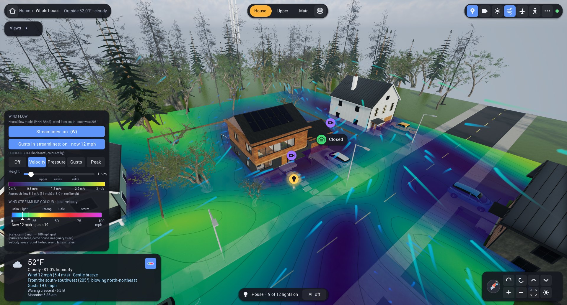
In an earlier post I described a live digital twin of my home, shown through an invented demonstration house so that nothing private appears on the page. This post covers the next step. I moved my own twin from a lightweight engine to Unreal Engine and rebuilt the demonstration house with every feature of the real one, including new pitched roofs, so that the pictures here show what the upgraded twin does.
It now looks and lights like a modern game. The HUD is comfortable on a phone held sideways, aircraft picked up by an ADS-B receiver fly over the house, and the wind comes from a physics-informed neural network (PINN), which drives the streamlines, the moving gust fronts and the contours of velocity, pressure and gusts around the house, its neighbours and its trees.
The part I learned most from was the validation. Trained on physics alone, the model got surface pressures wrong by a factor of three to five. Large-eddy simulation (LES) reached the guideline's hit-rate level on an isolated building, yet it did not measurably improve the network's surface pressures. The teacher that could handle neighbours turned out to be a cheaper, tunable turbulence model called GEKO. On a dense wind-tunnel array of houses it cut the network's error by more than a factor of four, and by about two on a sparser one, and none of those measurements were used in training. That is a real improvement but only a partial pass, and the rest of this post shows both sides against the measurements.
About the images
The twin runs in my own home, but for privacy the house in this article is not real. The pictures and the film show a generated stand-in, the “Imaginary House”, on a fictitious Seattle street, rendered by the same software with simulated data. Neither this house nor mine has wind measurements, so the wind model is validated on public wind-tunnel experiments on similar buildings.
The real house
In my own home, everything the twin shows is live. Flight data come from a local receiver, and the sensors and controls are all on the local network, which I can also reach from outside over the internet. Two things are not measured at the house, though. An aircraft's type and route are looked up in a public database, and the wind around the house is the model's estimate from the live weather feed.
From a model to a world
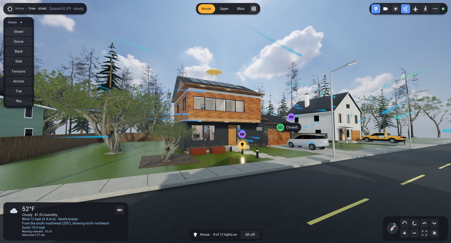
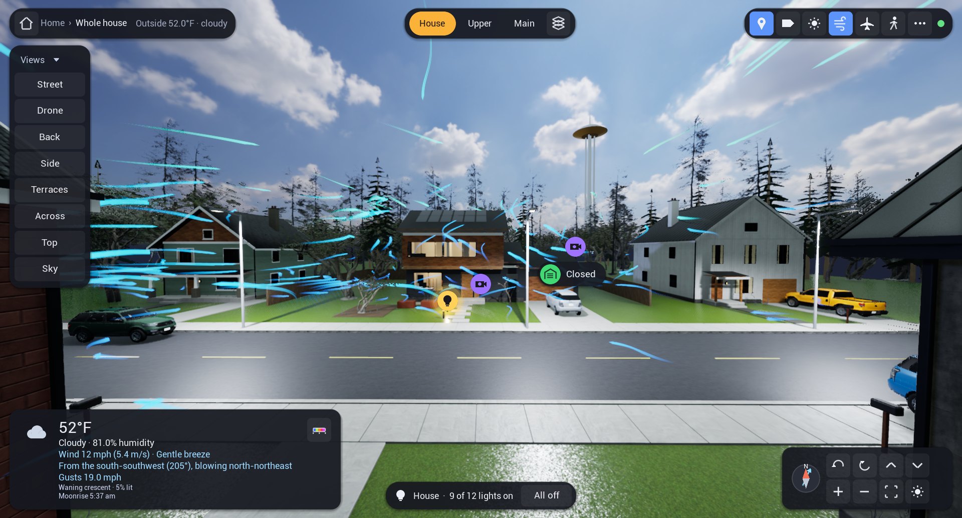
The games I played as a kid had a particular magic: a small, complete world you could fly a camera over, where the light moved with the time of day, the weather changed and little things happened on their own. That was the feeling I wanted the twin to have, and it is what a game engine is built to deliver. Unreal Engine gives the house physically based materials, soft shadows from a sun that stands where it really stands, a sky lit from a high-dynamic-range photograph and captured in real time so the shaded side of the house is never black, and detailed tree models instead of cones on sticks.
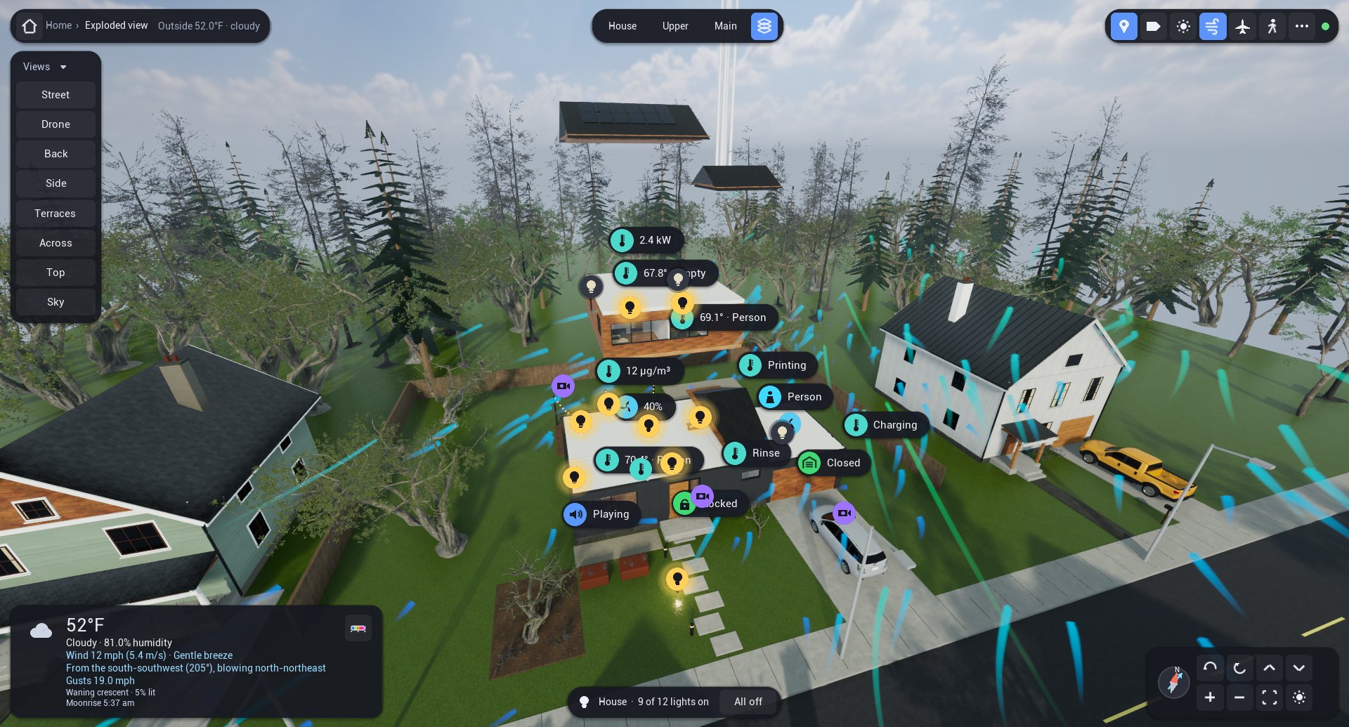
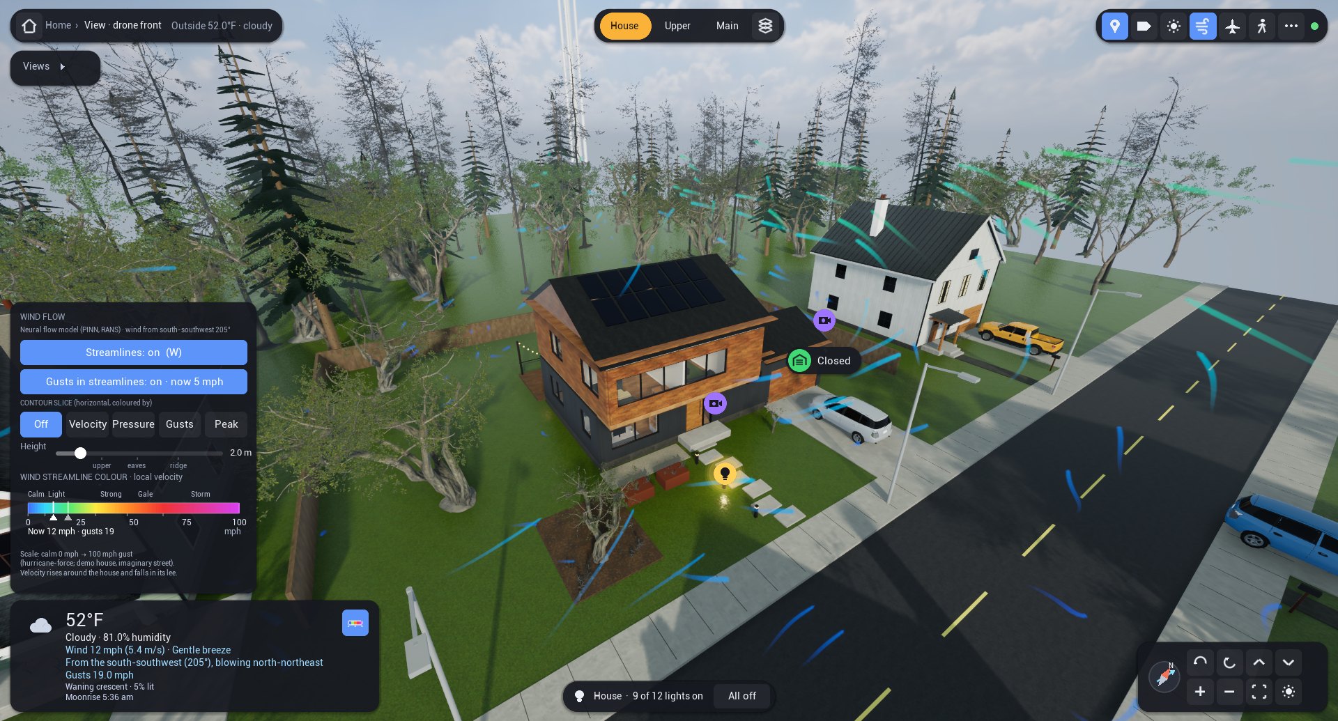
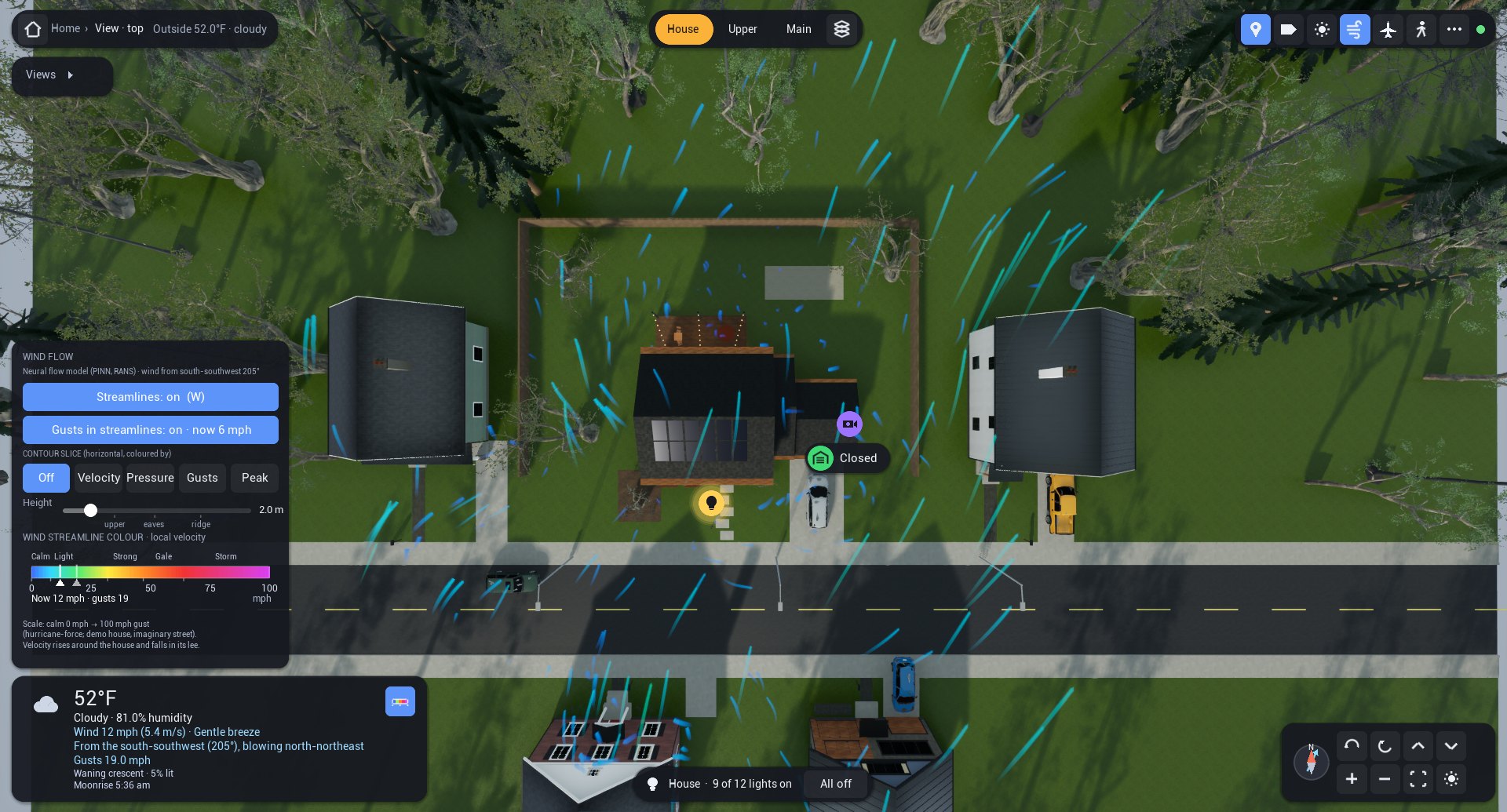
The house is still built in code rather than from a hand-made 3D file, so every wall, window and device stays addressable. It is the same invented Seattle home as before, with a charcoal board-and-batten main floor, a cedar upper floor cantilevered over the entry and a back deck with string lights. Two things changed. I took out the tall fir in the front yard, because it hid too much of the house. And the flat roof, clerestory and green roofs became 6:12 gables with the solar array on the south slope, which matches the shape of the buildings tested in the wind tunnel and gives the wind a real roof to follow.
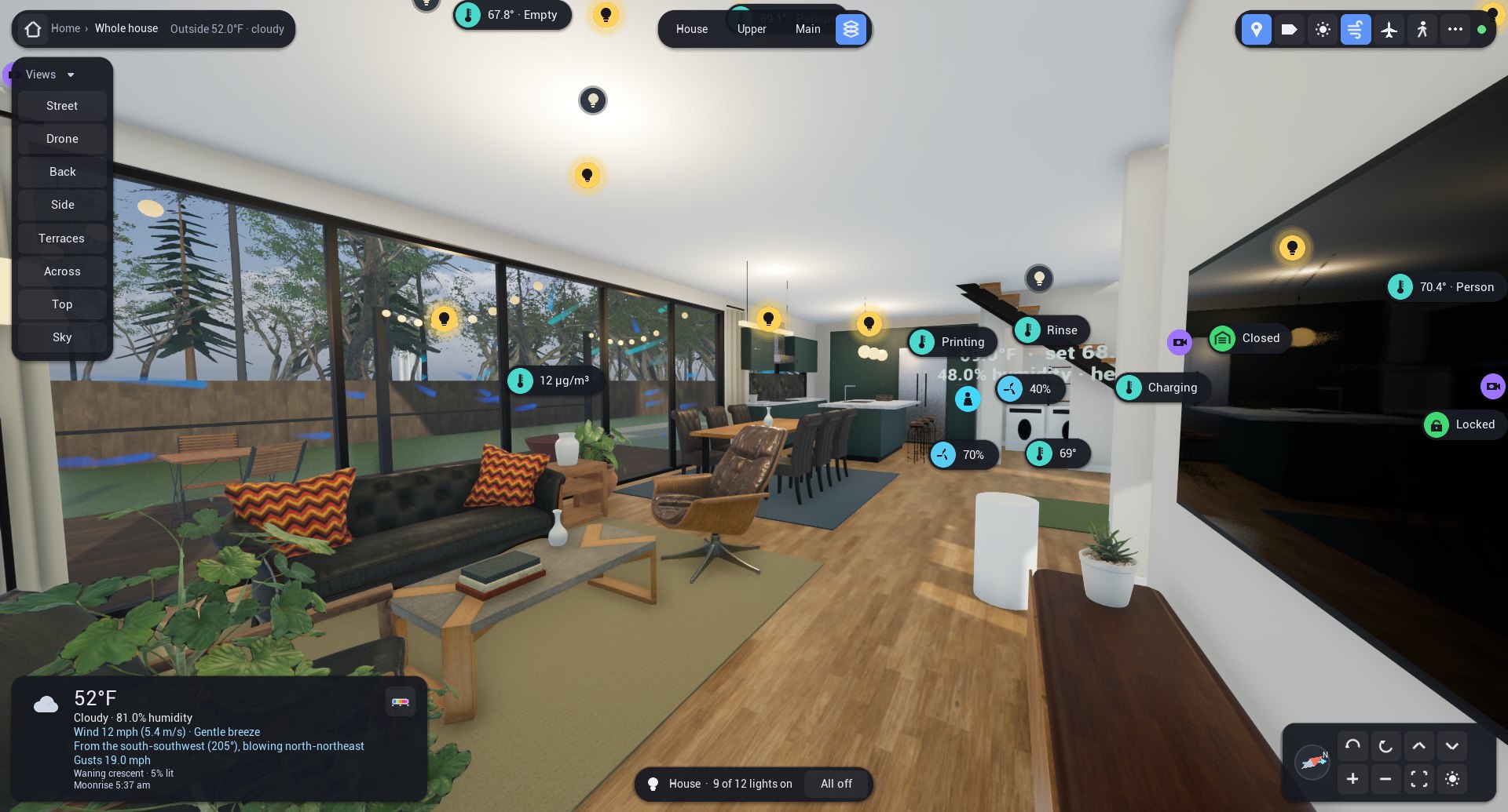
A HUD for the phone
The first version's interface was designed on a desktop and then squeezed onto the phone. This time I rebuilt the head-up display as an immediate-mode overlay that the engine draws directly every frame, scaled to whatever screen it is on: twice the size on a phone in landscape, larger on a tablet, and adjustable from the menu. On a short screen the views list collapses, the weather box goes compact, and long cards scroll instead of running off the edge.
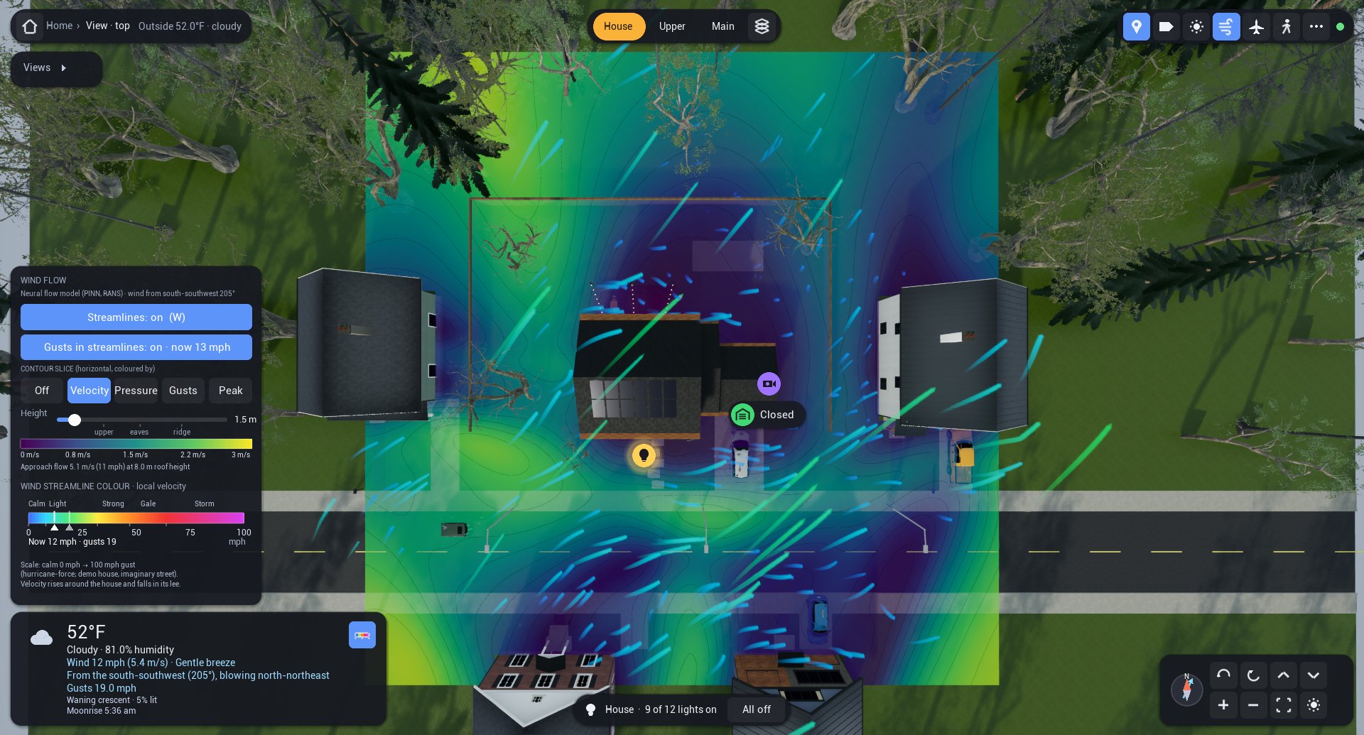
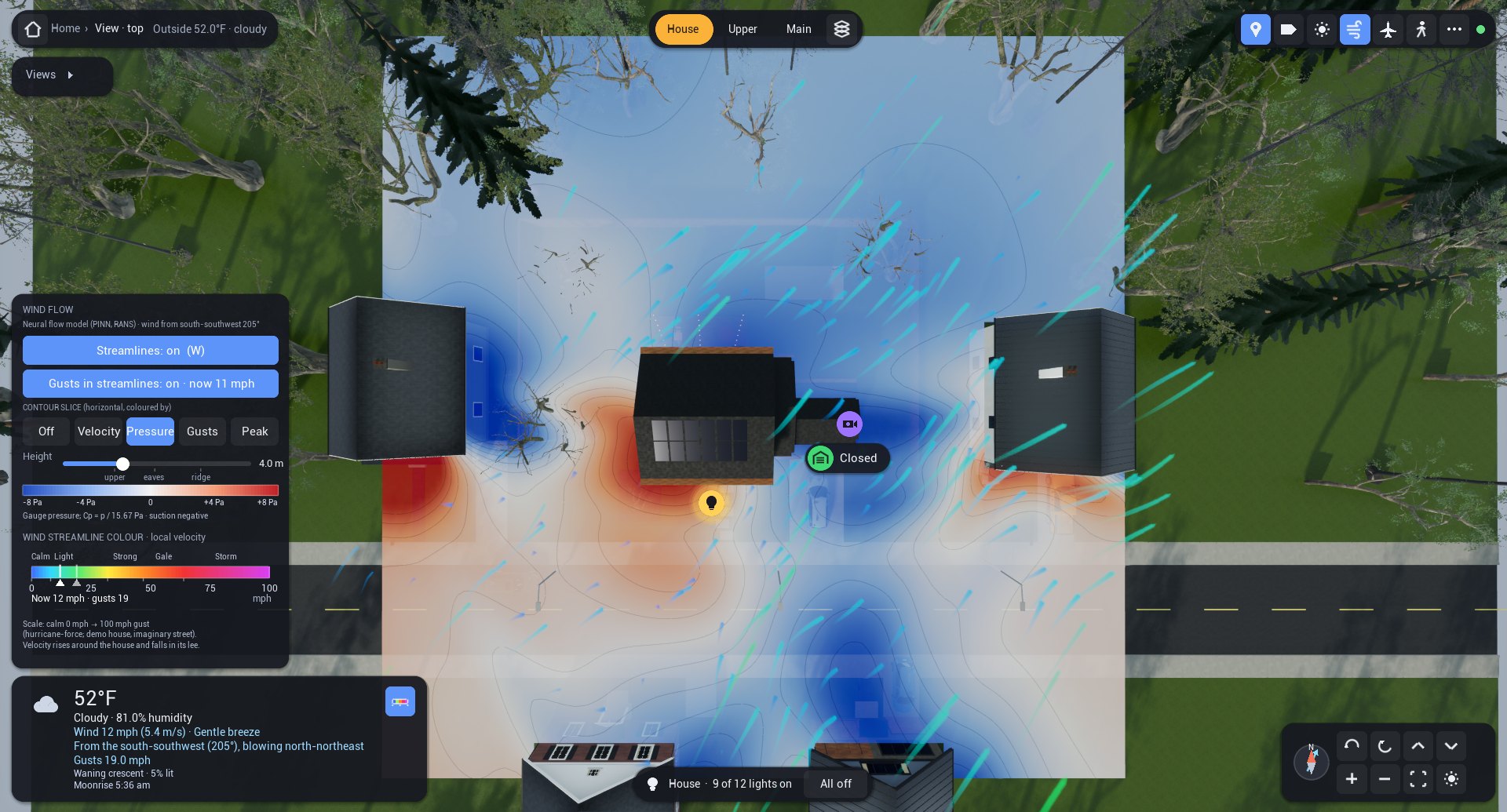
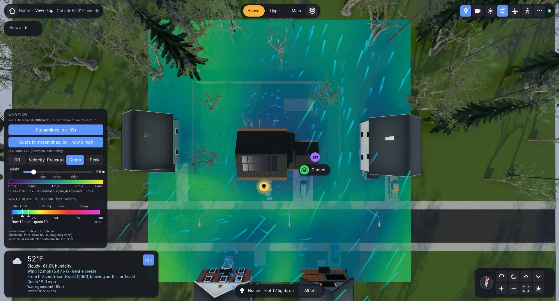
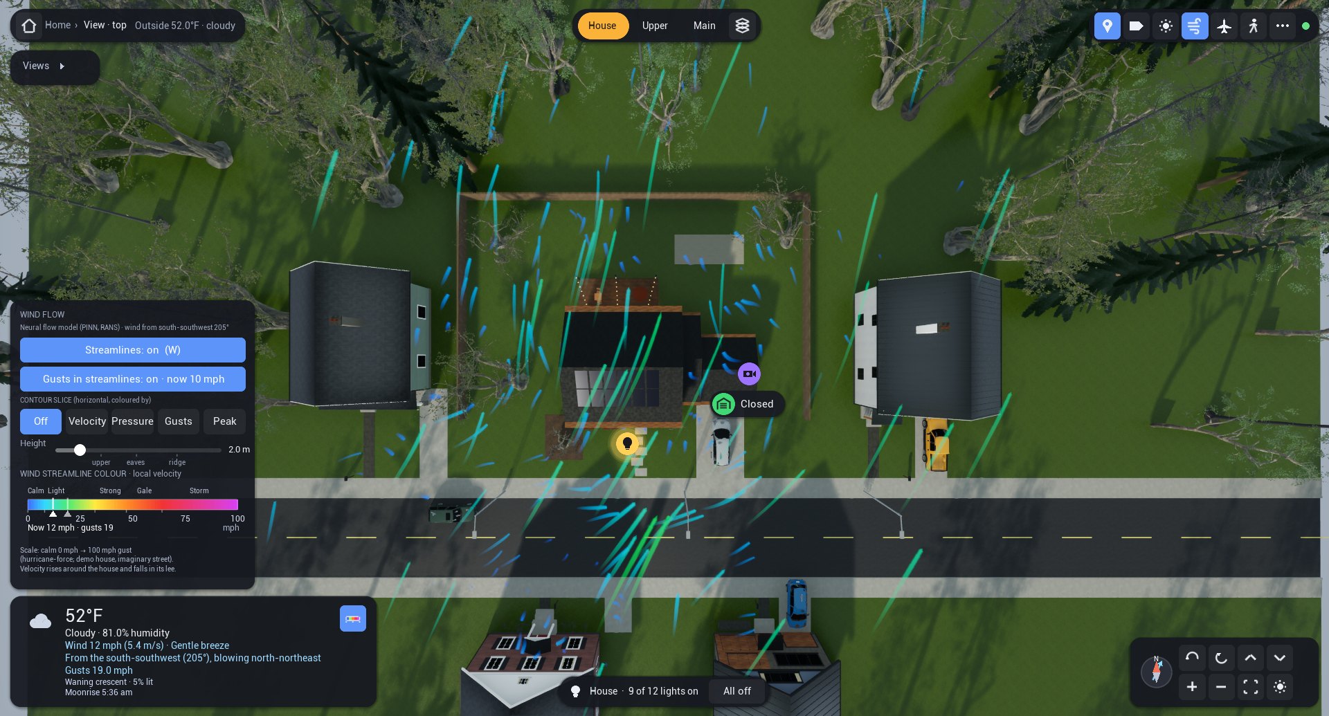
Along the top is where you are, the outside weather, the floor tabs (House, Upper, Main), the exploded view, and toggles for device markers, labels, day and night, wind, the sky view and walking. Device badges float over the model. Tapping a light or switch toggles it; tapping or holding any other badge opens its card, with brightness, locks, the garage door, the thermostat, the speaker and the cameras. The weather box has the temperature, wind velocity and direction, gusts, sunrise and sunset and the moon, and its wind button opens the new Wind flow panel. That panel switches the streamlines on or off, and the gusts in them, with the current gust velocity. It sets a contour slice coloured by velocity, pressure or gusts, adds a peak-pressure overlay on the house, and has a slider that moves the slice from 0.3 to 12 m, with marks at the upper floor, the eaves and the roof, beside the colour scale in m/s or pascals.
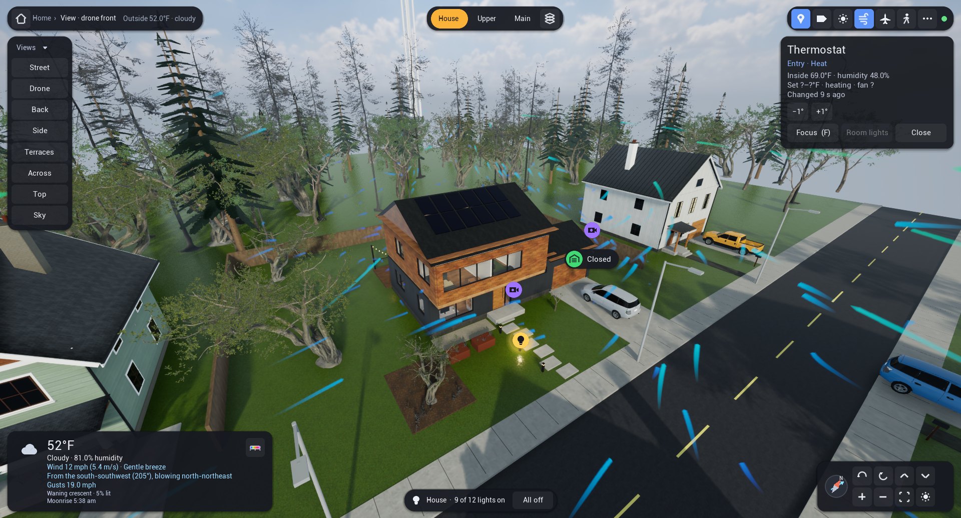
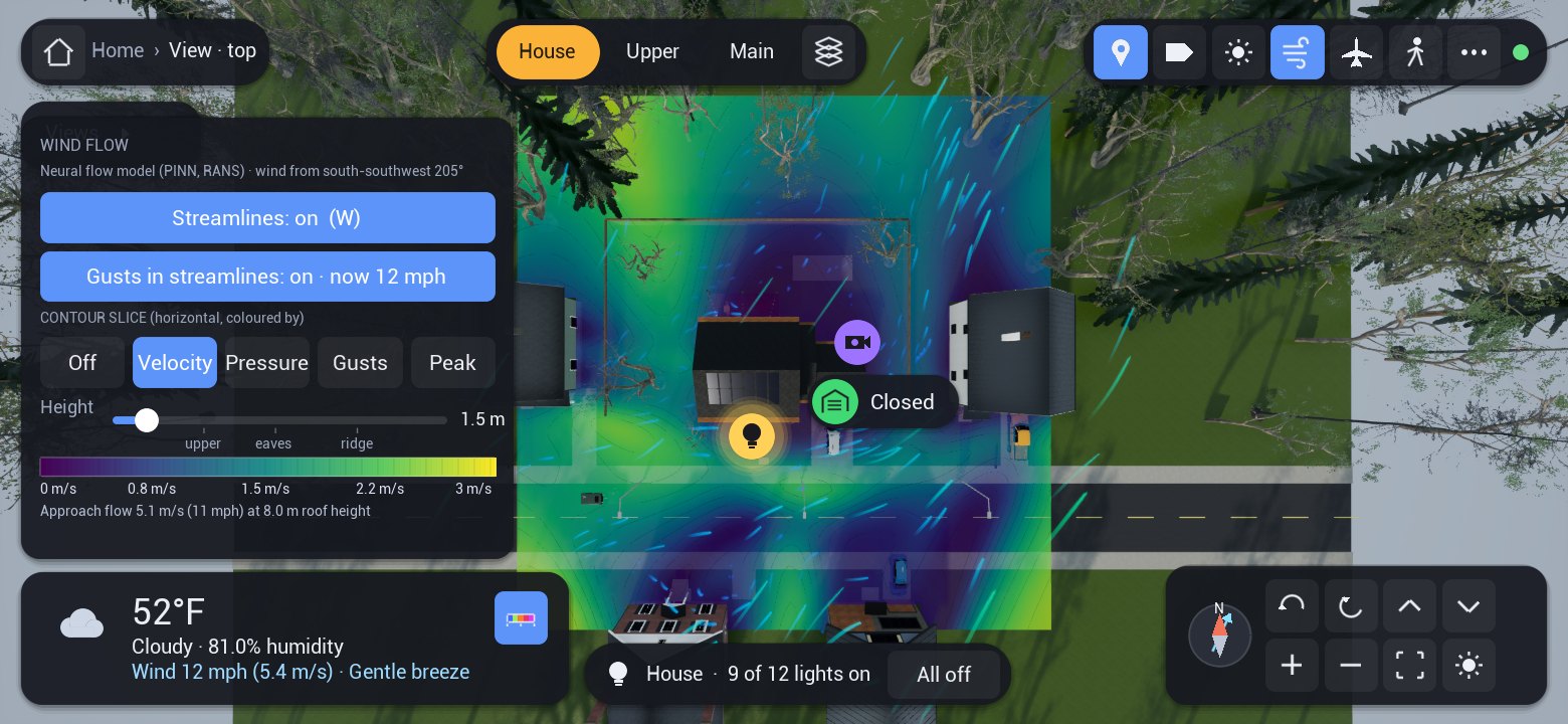
The whole twin runs on a phone
A modern Android phone runs all of this with no server apart from Home Assistant. It renders the world, receives the live data and evaluates the trained wind model itself.
The phone build draws the same house, street, trees and cars as the desktop and has the same peak overlay.
Aircraft overhead
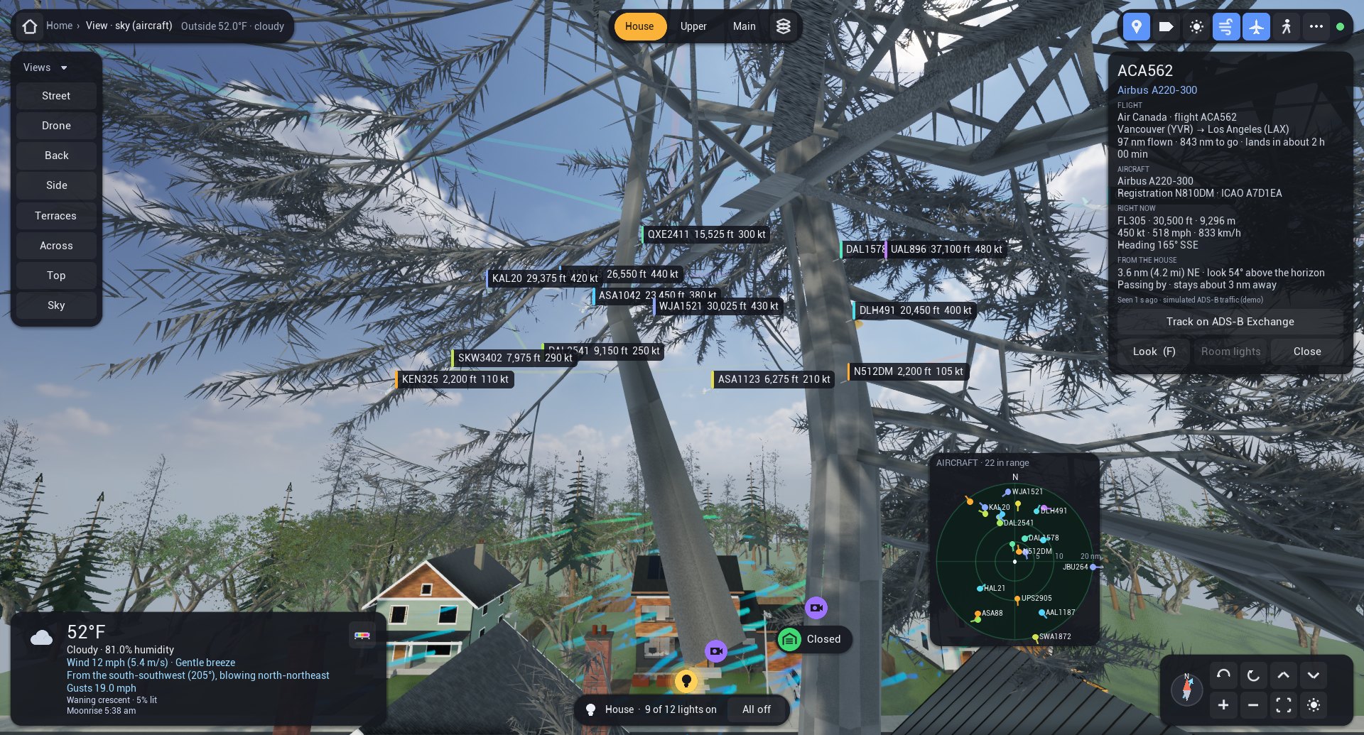
Aircraft fitted with ADS-B broadcast their position and velocity about twice a second, and their identity about every five seconds, on 1090 MHz. A small software-defined-radio receiver at my house decodes these messages, and Home Assistant turns the nearest aircraft into sensors carrying latitude, longitude, altitude, ground speed, track and a short trail. The twin reads those sensors and draws each aircraft in the sky above the house.
In the sky view each aircraft keeps its true bearing from the house, but its distance is compressed so that traffic twenty miles out still fits in the frame, and low aircraft are lifted a little to clear the trees. Each one is a 3D airliner with navigation lights, strobes and a fin coloured by altitude. It flies smoothly between radio reports by dead reckoning and pitches with its measured climb or descent. A callsign label follows it around, and a north-up radar scope in the corner shows the same traffic on rings at 5, 10 and 20 nautical miles from the house.
Tap an aircraft and its card opens with the type, registration, operator, altitude and climb rate, speed, heading and distance. In my own twin the type and route come from the public adsbdb.com database. Airline route data go stale, so before showing a route the twin checks that the aircraft is actually somewhere along it. The demonstration house shows simulated traffic around Seattle and says so; none of it is a real flight.
The wind model and its training
My first twin drew the wind with a textbook shortcut, smooth flow around a cylinder. It looked plausible, but it had no wake behind the house and no realistic pressure on the walls. This version uses a physics-informed neural network [1]. A normal neural network learns only from examples. This one is also penalised whenever its answer breaks the equations that govern air flow, so it has to agree with the physics and with whatever measurements it is given.
The equations describe the average wind, the flow you would see if you could blur out the gusts. Trees slow the air passing through their crowns, and turbulence is represented by a simple mixing model based on how fast the air is turning [5]. The network is built so that air can never pile up or vanish, which keeps the flow physically consistent everywhere. Wind direction is one of its inputs, so a single network covers every direction, and when the forecast wind gets stronger the whole pattern simply scales up.
Gusts are added on top. They come from a method called kinematic simulation [9], which sends random swirls of air along with the wind, sized and spaced to match wind-tunnel records. Each gust you see is a plausible example, not a forecast of a real one.
What did not work
Trained on the equations alone, the network kept settling on the wrong answer: a slow, swirling pocket of air in front of the house with almost no pressure build-up. The equations were nearly satisfied there, so the training had no reason to leave. The pressures it predicted on the walls were three to five times too weak. Adding the neighbouring houses to the model didn't fix it either. Physics alone was not enough. The network needed data.
Simulations as teachers
Wind tunnels measure pressure at small holes in the walls of scale models, but nobody has put these houses in a tunnel. A detailed computer simulation can fill that gap, as long as the simulation itself has been checked against experiments first. I used two kinds of flow simulation, both in the free OpenFOAM software.
Large-eddy simulation (LES) recreates the big turbulent swirls as they form and break up over time [10], [11]. It is the more detailed of the two and by far the more expensive. GEKO [6] works out only the average flow, which makes it quick enough to run with the neighbouring houses and trees for many wind directions, and its settings can be adjusted to fit experiments.
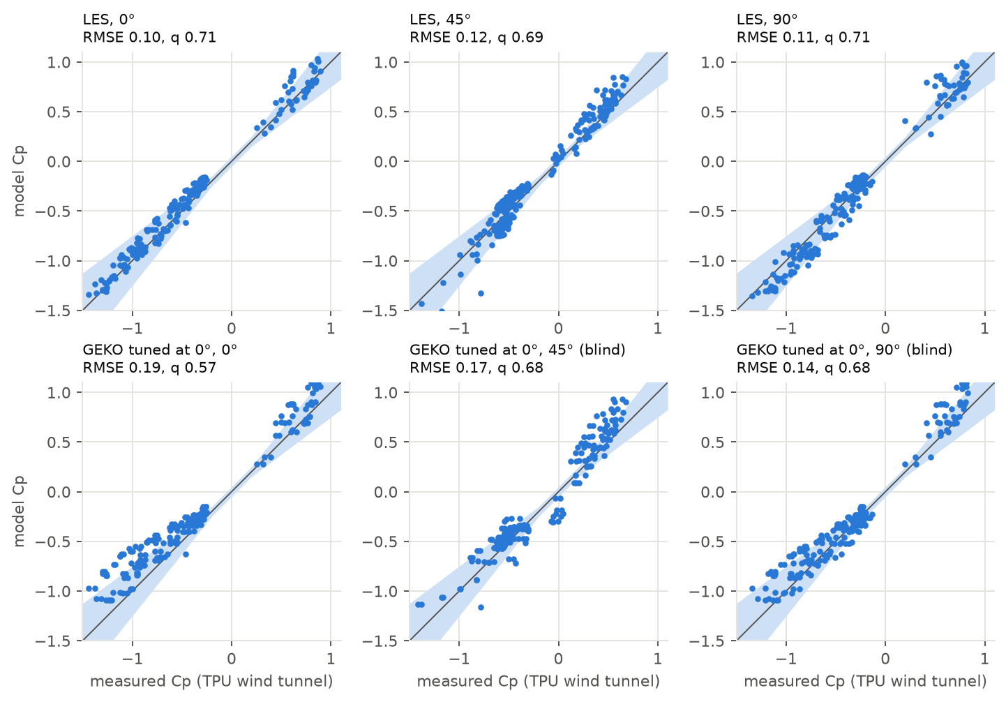
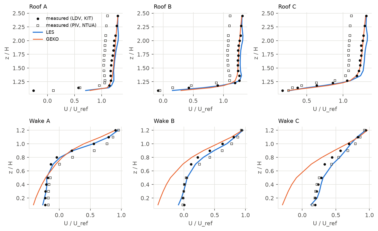
LES did three jobs. It checked the method on a flat-roofed building in the tunnel, where it predicted the pressure within the allowed margin at about 70 % of the measuring points for each of three wind directions. That passes the two-thirds bar described in the next section, though only modestly, and it needed a standard tunnel correction that I chose after seeing the first result. It also supplied the turbulence levels behind the gusts on my own house. Its third job was a test: I added LES results to the network's training data to see whether they improved the predicted pressures. Repeating the training three times showed that any gain was smaller than the run-to-run scatter, so I can't claim one.
GEKO was the teacher that mattered. Adjusting its settings to one building looked promising at first, but most of the gain went away when I checked it more carefully, and on a different layout the adjusted settings made two of the three wind directions worse. The houses therefore use GEKO's standard settings. On my own street, with no trees in either, GEKO and LES agree closely on the average wind, which only shows that the cheap simulation matches the expensive one. Whether either of them is right is something only measurements can tell.
Validation against experiments
How I keep score
I count a prediction as a hit when it falls within 25 % of the measured value, with a small fixed allowance where the measurement is close to zero, and I report the hit rate, the share of points that are hits. A model passes at two thirds (0.66). The idea comes from VDI 3783 Part 9 [4], the German engineering guideline for judging wind models around buildings, which the European COST 732 work also uses [7]. The guideline is written for wind velocities with a tighter allowance near zero. Applying it to pressures, with a looser allowance, is my own adaptation, so “pass” in this post means this adapted test, not formal compliance.
A hit rate on its own can mislead. It is harsh wherever the measured value is near zero, because 25 % of almost nothing is a very narrow target. So I also looked at the typical size of the misses and at whether the model rises and falls with the measurements. Where those tell a different story, I say so.
Isolated buildings, with data held out
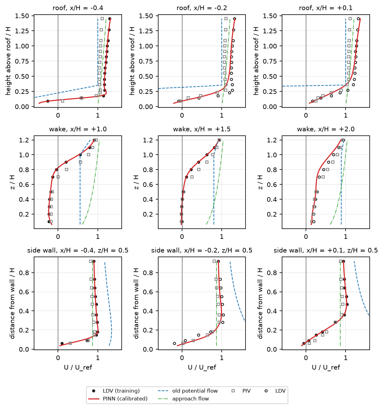
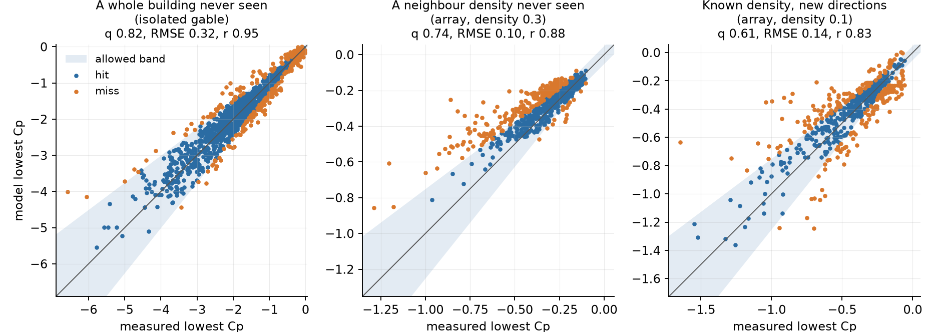
The measurements come from Tokyo Polytechnic University's TPU Aerodynamic Database [3], with wind-tunnel pressures at hundreds of points on scale buildings, and from the European TWEET-IE twin test, where the same cube was measured in two separate wind tunnels [2]. For each one I kept part of the data out of training and only used it to grade the network afterwards. On those unseen points, the network was a hit at 82 % of the held-out velocity points on the cube, which included every profile from the second tunnel, at 88 % of the pressure points on a gable-roofed building for wind directions it never saw, and at 84 % on a flat-roofed one. All three pass comfortably.
A building among neighbours
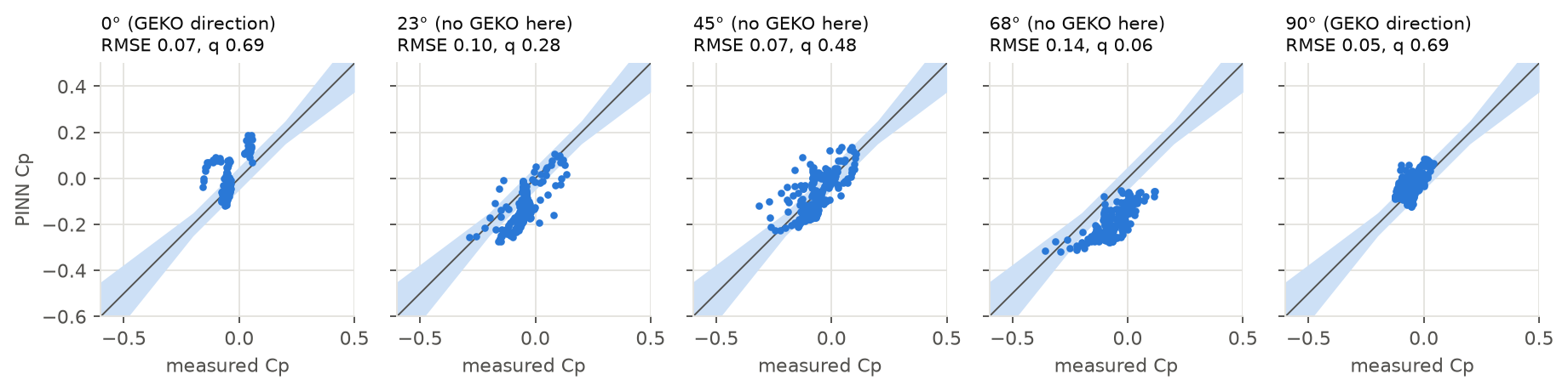
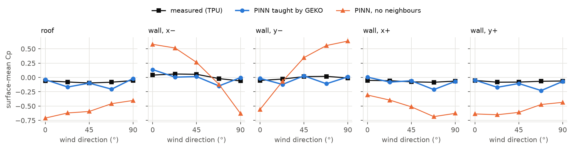
A real house has neighbours, and they shelter it. Tokyo Polytechnic also measured low-rise gable buildings laid out in regular grids [8], so I taught a network with GEKO results at a few wind directions and then graded it against the measured pressures on the building in the middle. None of those measurements went into training.
This is the result I care about most, and it is a partial pass. On the tightly packed grid, GEKO's teaching cut the typical error by more than four times compared with a network that knew about the neighbours but had no teacher, and by about six times compared with one that ignored them. The hit rate rose too, but it reached two thirds only at some of the directions the teacher had covered. Spacing the teacher's directions closer together, every 30° instead of every 45°, removed most of the failure at the worst direction. On a looser grid, closer to a suburban street, the error roughly halved, and there GEKO itself was the limit: the network was about as accurate as its teacher, and adding more directions helped only a little.
For trees, the closest experiment with measurements was the same cube with a layer of porous foam on its windward wall or roof [2]. GEKO with the foam treated as a drag zone came out slightly closer to the measurements than GEKO ignoring it, and on the roof it followed the measured change. That is modest support for how the model treats trees. Foam is not a tree, and how dense the tree crowns are is my assumption.
Why the experiments matter
It is easy to make a flow look right. The cylinder sketch looked convincing, and so did the physics-only network, until the measurements showed its pressures were three to five times too weak. A model earns trust by predicting measurements it has never seen: whole wind directions held back, and a second wind tunnel that tells you whether it learned the flow or just the quirks of one facility.
Some of this applies well beyond one house. Physics and data worked together where neither worked alone. A model trained on a simulation inherits that simulation's errors, and agreement between two simulations says nothing about reality. Settings tuned to one experiment didn't carry over to another. And a single training run once showed a benefit from LES that disappeared when I repeated it, so I now repeat a run before believing a gain.
07 · ResultsResults on the house
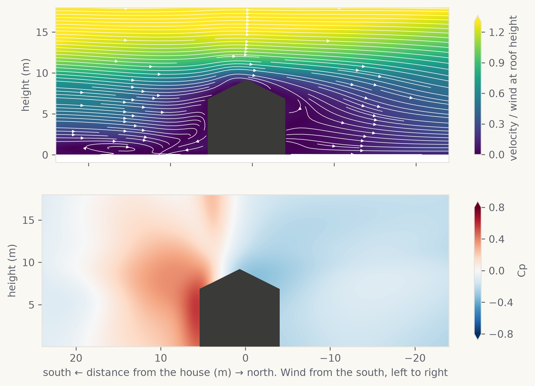
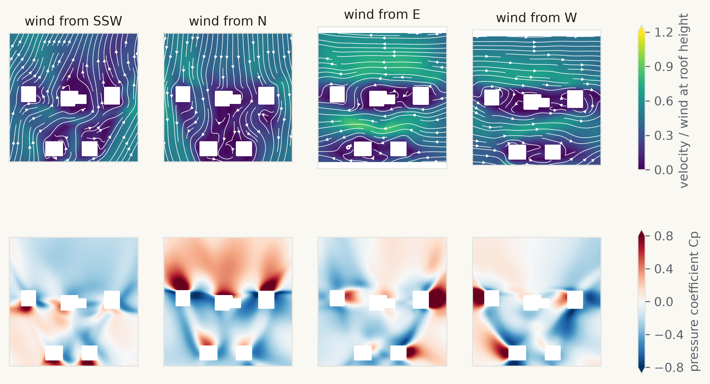
For the demonstration house I simulated the house, its four neighbours and 132 trees with GEKO for 12 wind directions, treating the trees as zones that slow the air, and taught a network on the results. My own house uses the same method with 24 directions. Two things on screen were added afterwards, purely for looks, and are not in the wind model: the neighbours’ porches and the woods behind the houses across the street.
At wind directions it wasn't trained on, the network reproduces GEKO's pattern well, but it is within the margin at only about half of the velocity points and a third of the pressure points on the house, below the two-thirds bar. Since that compares the network with its own teacher, it shows how well it fills in between directions and says nothing about reality.
In the app
Streamlines show where the air goes, and the coloured slice shows how fast it moves and how hard it pushes. The network discourages air from passing through walls but can't rule it out completely, so near a building the app steers the moving lines along the surface instead of into it, while their colours and the slice stay exactly as the model predicts. More of the lines start low down, so you see the wind at door and window height as well as over the roof. Across the whole film, none of the lines I sampled was inside a modelled building. Things that aren't in the model, like the porches and the parked cars, can still be crossed.
The slice can sit anywhere from ankle height to above the roof and shows velocity, pressure or gusts, where the gust value is the average wind plus three times its typical fluctuation. The demonstration house takes its turbulence from GEKO; my own takes it from LES. Checked against wind-tunnel records, the simulated gusts have the right strength and the right size, and the right ratio between a three-second gust and the average wind.
Peak pressures
The average pressure doesn't tell you what lifts a shingle. Brief peaks do, and they are much stronger. On the gable building in the tunnel, the strongest peak suction in a 10-minute record is about four times the strongest average. The network only knows averages, so a second, much simpler model estimates the peaks. It contains no flow equations: it learned directly from 134 wind-tunnel pressure records covering 20 building layouts, including gables of different sizes and roof pitches, a flat roof and grids of houses at three spacings. Given a point on a building, the wind direction and how closely packed the neighbours are, it returns the typical and extreme pressures there.
I graded it on buildings and layouts left out of training. It carries over well to buildings it has never seen, and it improved a lot with variety: trained on five building cases it was a hit at only 15 % of the points on an unseen gable, and trained on sixteen it reached 82 %. It beat a simple lookup of average values in every test. Its weak spot is the case that looks most like a suburban street, loosely spaced neighbours, where it stayed below the two-thirds bar. The size of the pressure fluctuations is its most reliable output.
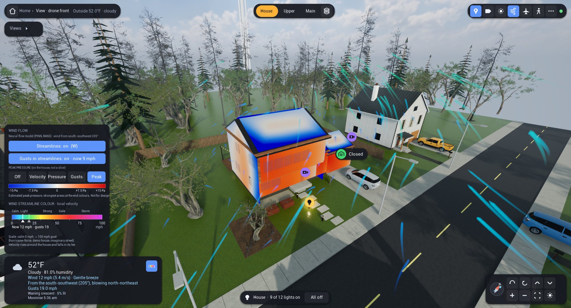
In the app, the Peak option colours every roof slope and wall in pascals, and the values grow with the square of the live wind, so doubling the wind quadruples them. The main block of the house is closest to the tunnel data. The wing and garage are an extrapolation, because no building in the data had attached wings, and the neighbours in the tunnel were all identical, which a real street isn't. The app's version gives the same numbers as the original model to five digits, and my own twin has the same option. Both are estimates borrowed from similar buildings in a wind tunnel, with no measurement at either house, and they are not for design.
08 · LimitsLimitations
Neither house has any wind measurements. Everything here was checked on similar buildings in a wind tunnel, whose approaching wind may not match the real site. Among neighbours the network passes only at some wind directions, and on a loosely spaced street its teacher sets the limit. The network gives the average wind; the gusts are realistic but random, so they can't predict a particular gust, and peak pressures come from the separate tunnel-based estimate. The tree density is assumed, the trees are placed by the app's forest generator, and sloping ground and roof overhangs are left out. GEKO also has a pressure offset on a single building that I still can't explain. Finally, the weather feed's wind at 10 m stands in for the wind arriving at the house, which is a rough assumption in a wooded suburb.
Disclaimer: why independent experimental validation is required
The wind results in this post have not been independently validated, and nothing here should be used for structural design, insurance, safety decisions or storm preparation. There are three reasons.
First, the tests are not independent. I chose the methods, the data splits, the scoring rule and its tolerance, with help from a language model, and in places I picked a correction after seeing the result. Holding data out reduces that bias but doesn't remove it; someone else, working blind, needs to repeat the comparison. Second, the experiments are not of these houses. Every measurement comes from a scale model of a similar building in a wind tunnel, and real sites have sloped ground, real trees, eaves and weather that a tunnel doesn't, so agreement there is evidence by analogy only. Third, a simulation can't stand in for a measurement. The app's network is taught by a simulation, and on the house it can only be scored against that same simulation.
What would settle it is a set of measurements at a real house, taken by someone other than the modeller and compared with predictions fixed in advance: a three-dimensional sonic anemometer for the wind and pressure sensors on the walls and roof, recorded through real storms. Next best would be a blind wind-tunnel test of the house's geometry with its neighbours.
Why vortex shedding is not modelled
Vortex shedding is the regular peeling of swirls off the sides of a building, the effect that can set tall, slender towers swaying. I left it out for three reasons. The tunnel records of these low, wide buildings show little of it, only a broad, weak signal that is probably just the slow gusts in the approaching wind. Simulating it properly would take days of computing for each wind direction, and the simulated inflow I have adds artificial disturbances that would blur exactly the effect I'd be looking for. And nothing at the house measures wind or pressure, so the result couldn't be checked. The gust model already includes a random wake behind the house, so the wake on screen is never still, but it is a statistical sample rather than a modelled row of swirls.
Closing thoughts
Moving to a game engine changed how the twin feels. It is now somewhere I actually want to look, on the phone as much as on the desktop. Replacing the wind illustration with a physics-informed model changed what the wind display means, and testing that model against measurements changed what I believe about it. I went in expecting the most expensive simulation to teach the network the most, and on this evidence it was the cheap one, checked against measurements, that did. The aircraft are just fun. I did much of the simulation, training and validation work in conversation with a large language model, and I now have a working digital twin of my house.
Assets. The furniture, plants and trees are CC0 models from Poly Haven, and the cars come from the free City Sample Vehicles pack for Unreal Engine.
Abbreviations
| Term | Meaning |
|---|---|
| ADS-B | Automatic Dependent Surveillance–Broadcast: aircraft radio position reports |
| CFD | Computational fluid dynamics |
| COST 732 | European Cooperation in Science and Technology, Action 732: best-practice work on urban flow simulation |
| Cp | Pressure coefficient: pressure relative to the dynamic pressure of the wind. Positive pushes on a surface, negative pulls |
| GPU | Graphics processing unit |
| DFSEM | Divergence-Free Synthetic Eddy Method: creates turbulence at the LES inlet |
| GEKO | Generalized k–ω: a steady turbulence model with tunable coefficients |
| HDRI | High-dynamic-range image |
| HUD | Head-up display: the interface drawn over the 3D view |
| KIT | Karlsruhe Institute of Technology |
| k–ω | Turbulence model family using turbulent kinetic energy (k) and its specific dissipation rate (ω) |
| LDV | Laser Doppler velocimetry |
| LES | Large-eddy simulation: resolves the large turbulent eddies in time |
| NTUA | National Technical University of Athens |
| OpenFOAM | Open-source Field Operation And Manipulation: the simulation software |
| PBR | Physically based rendering |
| PINN | Physics-informed neural network |
| PIV | Particle image velocimetry |
| RANS | Reynolds-averaged Navier–Stokes: equations for the time-averaged flow |
| RMS | Root mean square: here, the size of pressure or velocity fluctuations |
| RMSE | Root-mean-square error: the typical size of a model’s miss |
| σu, σw | Standard deviation of the along-wind and vertical velocity |
| TPU | Tokyo Polytechnic University, whose wind-tunnel database is used here |
| TWEET-IE | Twin Wind tunnels for Energy and the Environment: Innovations and Excellence, a European project |
| Uref | Reference wind velocity that all velocities are divided by |
| VDI | Verein Deutscher Ingenieure, the Association of German Engineers, which publishes guideline VDI 3783 |
| WALE | Wall-Adapting Local Eddy-viscosity: the LES subgrid model |
References
- M. Raissi, P. Perdikaris, G. E. Karniadakis (2019). Physics-informed neural networks. Journal of Computational Physics 378, 686–707. doi:10.1016/j.jcp.2018.10.045
- V. Pappa, C. Gromke, D. Bouris (2023). Twin test 1: Effect of vegetation on urban flows. PIV data from NTUA WT experiment and LDV from KIT WT experiment. Zenodo, CC BY 4.0. doi:10.5281/zenodo.10019002
- Tokyo Polytechnic University (TPU), Wind Engineering, TPU Aerodynamic Database: low-rise buildings without eaves, cases g080427 (gable) and g080600 (flat). db.wind.arch.t-kougei.ac.jp; Y. Quan, Y. Tamura, M. Matsui, S. Y. Cao, Y. Yoshida (2007). TPU aerodynamic database for low-rise buildings. Proc. 12th International Conference on Wind Engineering, Cairns, 1615–1622.
- VDI 3783 Part 9 (2017). Prognostic microscale wind field models: evaluation for flow around buildings and obstacles. Verein Deutscher Ingenieure.
- M. Kato, B. E. Launder (1993). The modelling of turbulent flow around stationary and vibrating square cylinders. Proc. 9th Symposium on Turbulent Shear Flows, Kyoto.
- F. R. Menter, A. Matyushenko (2025). Generalized k–ω (GEKO) two-equation turbulence model. AIAA Journal 63(11), 4590–4606, as cited in the OpenFOAM v2606 release notes.
- J. Franke, A. Hellsten, K. H. Schlünzen, B. Carissimo (2011). The COST 732 Best Practice Guideline for CFD simulation of flows in the urban environment: a summary. International Journal of Environment and Pollution 44, 419–427. doi:10.1504/IJEP.2011.038443
- Tokyo Polytechnic University (TPU), Wind Engineering, TPU Aerodynamic Database: non-isolated low-rise buildings. db.wind.arch.t-kougei.ac.jp
- J. C. H. Fung, J. C. R. Hunt, N. A. Malik, R. J. Perkins (1992). Kinematic simulation of homogeneous turbulence by unsteady random Fourier modes. Journal of Fluid Mechanics 236, 281–318. doi:10.1017/S0022112092001423
- F. Nicoud, F. Ducros (1999). Subgrid-scale stress modelling based on the square of the velocity gradient tensor. Flow, Turbulence and Combustion 62, 183–200. doi:10.1023/A:1009995426001
- R. Poletto, T. Craft, A. Revell (2013). A new divergence free synthetic eddy method for the reproduction of inlet flow conditions for LES. Flow, Turbulence and Combustion 91, 519–539. doi:10.1007/s10494-013-9488-2