AeroFlow NS is a real-time 3D wind-tunnel simulation that lives entirely inside a single HTML file. The remarkable part: the entire thing, the aircraft geometry, the fluid solver, the GPU particle system, the streamline tracer, the rendering pipeline, and the UI, was generated by Kimi K3, Moonshot AI's 2.8-trillion-parameter model, from a natural-language description.
No CAD file was imported. No mesh was loaded. No solver library was linked. K3 wrote the geometry as procedural signed distance functions, wrote the fluid solver from scratch, wired it into a Three.js scene, and packaged everything into a lightweight file you can open in any modern browser.
Disclaimer: This is a technology demonstration of what an AI model can generate, not a validated CFD tool. Treat it as a physically plausible real-time visualization, not a certified aerodynamic analysis.
Launch a simulation
Both simulations are standalone HTML files. Click a button below to open one in a new tab, no install, no plugin, no setup. Each runs the same fluid solver around a different procedurally-generated aircraft.
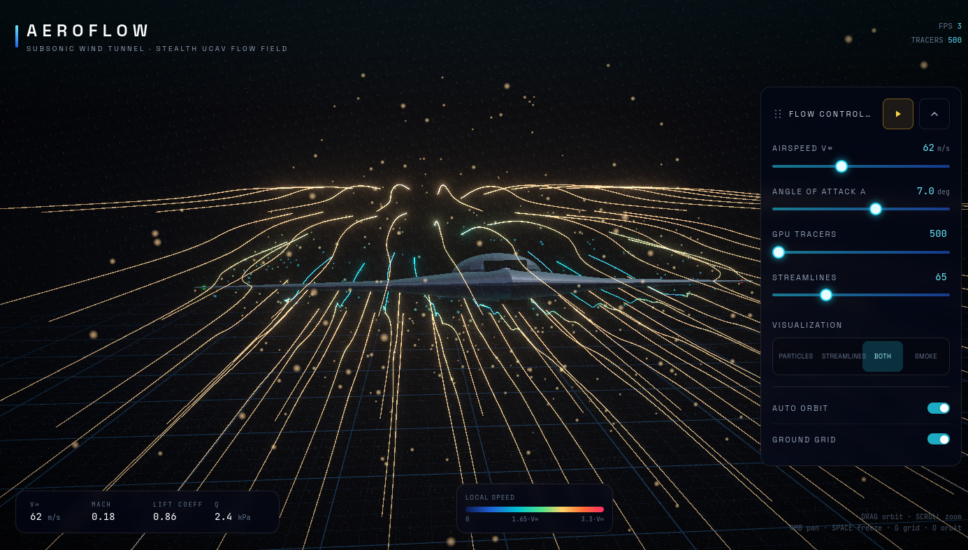
Stealth UCAV
Blended flying-wing with lambda planform and flat-shaded skin. Lower aspect ratio (AR = 4.2) produces wider, more intense wingtip vortices.
Open in new tab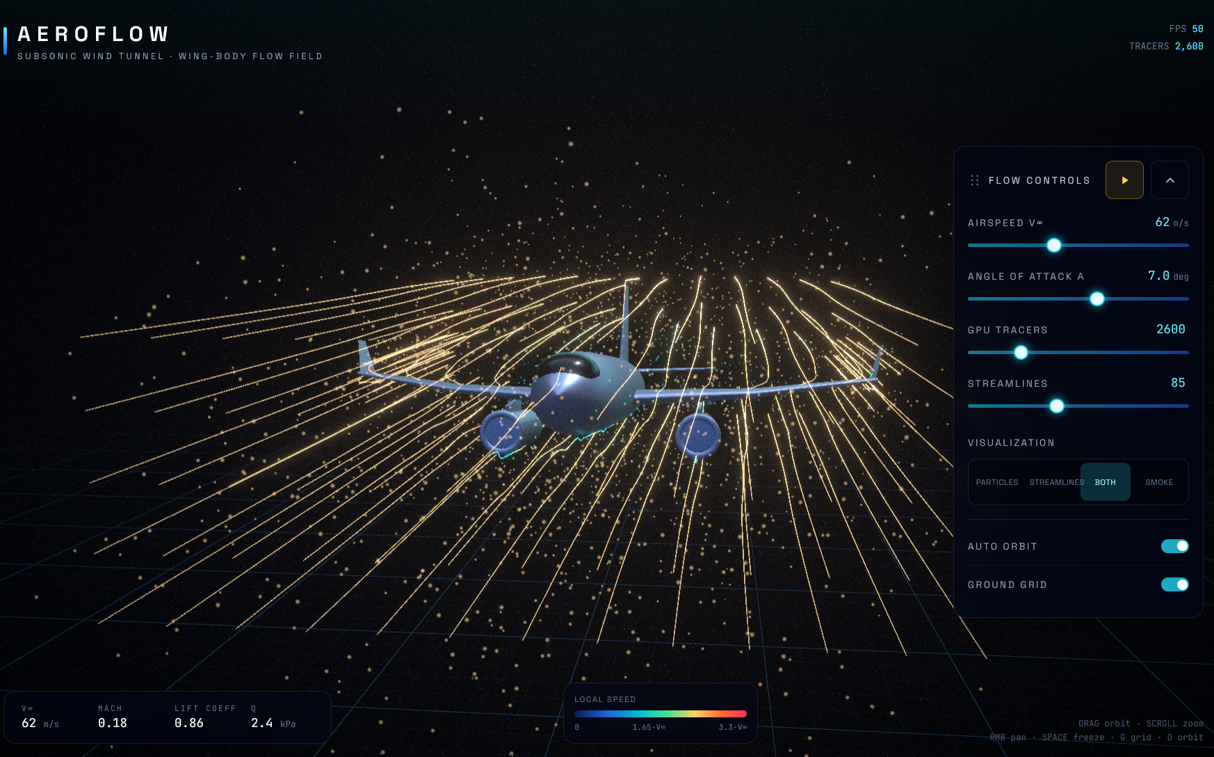
Refined Airliner
Jet airliner with winglets, engine nacelles, and stabilizers. Higher aspect ratio (AR = 5.14) produces tighter, more concentrated wingtip vortices.
Open in new tabQuick start once it's open
- Drag to orbit, scroll to zoom.
- HUD sliders: freestream velocity (default 62 m/s), angle of attack (default 7°), GPU tracer count (500–10,000), streamline count (10–200).
- Modes: particles, streamlines, both, or smoke.
- Keyboard:
Spacefreeze/resume,Ggrid,Oauto-orbit. - Try this: push angle of attack to 12°+ and watch the wingtip vortices intensify. Switch to smoke mode to see the wake as a continuous flow field.
What Kimi K3 generated
The entire simulation was produced by a single AI model from a natural-language prompt. Here is what K3 built, with no human-written code in the loop:
- Procedural aircraft geometry. Two complete aircraft, a refined jet airliner and a stealth flying-wing UCAV, generated from analytic signed distance functions. No CAD file, no mesh import, no asset pipeline. The fuselage, wings, winglets, engine nacelles, stabilizers, and tail are all described by mathematical formulas that K3 wrote.
- A real-time fluid solver. K3 wrote an incompressible fluid solver from scratch, the kind of code that normally takes a CFD engineer days to implement. It runs every frame in the browser, computing how air moves around the aircraft, and produces emergent features like wingtip vortices and wake structure without any of them being prescribed.
- GPU particle system. Up to 10,000 tracer particles, rendered in a single GPU draw call, color-mapped by local speed. K3 wrote the custom shaders, the advection logic, and the real-time count slider.
- Streamline tracer. 10–200 integrated flow lines, seeded upstream and around the wingtip vortex cores, colored by local speed.
- Smoke visualization mode. A fourth render mode that turns the same particles into soft, diffuse puffs, evoking smoke or dye in a real wind tunnel.
- Full rendering pipeline. Three.js scene, React Three Fiber integration, bloom/noise/vignette post-processing, HUD controls, loading splash, and WebGL fallback.
- Standalone HTML packaging. K3 configured the build to inline everything, code, fonts, shaders, into a single ~2.2 MB HTML file. No server, no dependencies, no install.
Lightweight by design
The most striking thing about AeroFlow NS is its delivery format. A real-time 3D fluid solver with procedural geometry, GPU particles, and post-processing, and the entire thing is one HTML file:
- ~2.2 MB per aircraft. Everything inlined: solver, geometry, shaders, fonts, UI. No external requests at runtime.
- Open in any modern browser. Chrome, Firefox, Safari, Edge, if it has WebGL, it runs.
- No install, no plugin, no server. Double-click the file or host it anywhere static. It just works.
- 60 FPS on a modest GPU. The solver is tuned for real-time: a coarse but stable grid, unconditionally stable advection, and a loose pressure solve that converges in 18 iterations.
- Two files, one solver. The airliner and the UCAV share the identical solver: only the geometry SDFs and rendering materials change between them.
Why this matters
Traditionally, sharing a CFD result meant shipping a multi-gigabyte dataset, a ParaView install, or a rendered video. Kimi K3 collapsed all of that into a single HTML file that anyone can open and interact with. The simulation is not a recording: it is a live solve, running on the reader's own GPU, the moment they click the link.
Two aircraft, one solver
Both models run the identical fluid solver: only the procedurally-generated geometry and the rendering materials change:
| Model | Geometry (procedural) | Aspect ratio |
|---|---|---|
| Refined airliner (v2) | 19-station lathe fuselage, 4-station lofted wings + winglets, stabilizers, vertical tail, engine nacelles with fan discs | AR = 5.14 |
| Stealth UCAV | Blended flying-wing, 5-station lofted lambda planform (center chord 8.1 m → tip 1.0 m), cockpit/sensor box, exhaust slot, edge strips, sensor dome | AR = 4.2 |
- Same solver, different physics. The UCAV's lower aspect ratio and flying-wing planform produce wider, more diffuse wingtip vortices and a broader wake.
- The airliner's higher aspect ratio and distinct wing-fuselage junction create tighter, more concentrated vortices that persist further downstream.
- None of this is prescribed. The vortex structure emerges from the geometry interacting with the solver, exactly as it would in a real CFD calculation.
What emerges from the solver
Given only the freestream velocity, the geometry, and the angle of attack, the solver produces, with no prescribed inputs:
- A stagnation point at the nose of the aircraft
- Acceleration over the wing suction side
- A momentum-deficit wake behind the aircraft
- Two counter-rotating wingtip vortices that roll up from the pressure difference across the wingtips
- Downwash behind the wing
None of these are injected from a formula. They are all consequences of the solver running on the geometry. Change the angle of attack and the flow restructures in real time.
About Kimi K3
The entire simulation was produced using Kimi K3, Moonshot AI's most capable model. Key facts:
- 2.8 trillion parameters, at the time of writing, the world's first open 3T-class model.
- 1-million-token context window, enough to hold an entire codebase in working memory.
- Native vision, can leverage screenshots and live previews to refine visual output until the simulation looks right, not just computes right.
- Built for long-horizon coding, a single agent sustaining a complex engineering task across many files with minimal human oversight.
- Open weights, for nine of the past twelve months, Kimi models have set the upper bound of open-model sizes.
Why K3 was the right tool
AeroFlow NS sits squarely in the intersection of skills where K3 excels:
- 3D reasoning + coding. The airframe geometry requires spatial intuition, understanding how a trapezoidal wing planform maps to a 3D slab, how dihedral and thickness taper interact, and how the angle-of-attack rotation connects the wind and body frames.
- Numerical methods literacy. Writing a stable, correct fluid solver requires deep familiarity with the CFD literature, the right advection scheme, the right pressure solve, the right boundary conditions.
- Full-stack integration. The same agent wrote the solver, wired it into React components, configured the single-file build, inlined fonts as base64, and produced a LaTeX physics document.
- Vision-in-the-loop iteration. K3 refined particle counts, color palettes, bloom intensity, and camera framing by looking at the output, not just reading error messages.
An honest assessment
Having worked with CFD solvers and reviewed AI-generated code for years: K3 produced a genuinely decent model, one of the better AI-generated physics implementations I've seen.
- Right architectural choices: staggered grid layout, stable advection scheme, pressure projection, immersed-boundary geometry. Numerically stable, correct boundary conditions, physically plausible emergent features.
- Known limitations: coarse grid (0.5 m cells), loose pressure convergence, first-order advection smears fine features, no turbulence modeling.
- What a production solver would need: multigrid pressure, higher-order advection, boundary-layer resolution, turbulence modeling.
But as a real-time, browser-based demonstration of genuine fluid physics, generated by an AI model from a natural-language description, delivered as a single HTML file: it is remarkably competent.
The wingtip vortices you see trailing behind the aircraft are not injected from a formula. They emerge from the pressure difference between the upper and lower wing surfaces, exactly as they would in a real CFD calculation.
The bigger picture
The distance between "describe what you want" and "running simulation" is collapsing. Geometry, solver, rendering pipeline, UI, each piece would have taken days of expert work not long ago. With Kimi K3, the loop is: describe the physics, review the output, refine. The model handles the implementation, the integration, and the build.
The question isn't whether AI can produce a simulation like this from a single command. It's how soon "a single command" becomes the boring part, and the interesting work moves to what you ask for next.
Technical summary
| Component | What K3 generated |
|---|---|
| Geometry | Procedural signed distance functions, no CAD, no mesh import |
| Solver | Real-time incompressible fluid solver, 52×26×36 grid, 60 FPS |
| Particles | GPU points, 500–10,000 controllable via slider, single draw call, custom shaders |
| Streamlines | 10–200 controllable, 4th-order Runge-Kutta integration, adaptive step size |
| Smoke mode | 4th visualization mode, soft, diffuse puffs evoking wind-tunnel dye |
| Rendering | Three.js, React Three Fiber, bloom/noise/vignette post-processing |
| Controls | HUD sliders (velocity, angle of attack, tracers, streamlines), 4 mode toggles, keyboard shortcuts |
| Delivery | Two standalone HTML files, ~2.2 MB each, all assets inlined, open in any browser |
If you found this interesting, you may also enjoy the companion posts on LLM-orchestrated CFD and why external aerodynamics is the easy part.