This release marks a step forward for Turbulence Realm SINDy and Tracker. SINDy now offers six distinct methods for discovering governing equations from video, while Tracker has grown from a simple region-clicking tool into a full analysis console for bubble-laden and multiphase flows. Both run as ordinary installers on Windows and Linux, with every major dependency included.
New alongside this release is AeroFlow NS, a real-time 3D Navier-Stokes wind tunnel that runs entirely in your browser. Two procedural aircraft (a refined airliner and a stealth flying-wing UCAV) are built from signed distance fields, solved on a staggered MAC grid every frame, and visualized with controllable GPU tracers, smoke flow visualization, and adaptive streamlines. Both simulations are embedded and fully interactive further down this page.
Why six methods, not one?
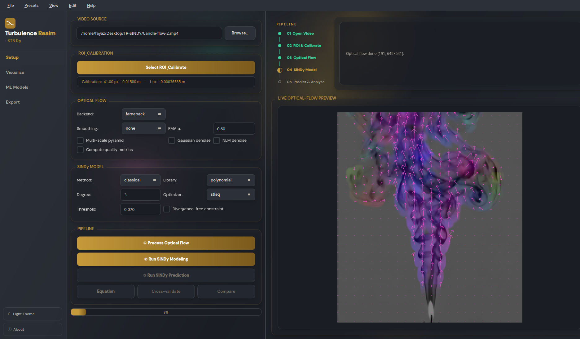
SINDy is a powerful idea: watch a video, extract motion, and let the software discover the simplest equation that explains what it sees. The catch is that fluid motion comes in many forms. A purely polynomial model can miss the physics when the data is noisy, when the equation has a denominator, or when the experiment is actively driven by a pump or actuator.
Instead of forcing a single algorithm to handle every situation, the new SINDy Model card gives you a dropdown with six sparse-regression methods. Choose the one that matches your data, and the interface adapts automatically.
| Method | What it does | When to use it |
|---|---|---|
| Classical SINDy | Discovers clean, explicit equations from smooth data | Your default starting point |
| SINDy-PI | Handles rational and implicit equations | The equation has fractions or unknown denominators |
| PDE-FIND | Discovers partial differential equations | You have spatial grid data, not just time series |
| WSINDy | Uses weak forms to resist noise | Your data is rough, sparse, or low quality |
| E-SINDy | Runs an ensemble and keeps only the consistent terms | You need robust results from limited data |
| SINDYc | Includes external forcing or control inputs | Your flow is driven by pumps, valves, or actuators |
What this means in practice
If you have a clean video of a vortex street, Classical SINDy may give you the equation in seconds. If your video has pump-driven forcing, switch to SINDYc. If the data is grainy, try WSINDy or E-SINDy. The right method is now one click away.
Cross-validation that keeps going
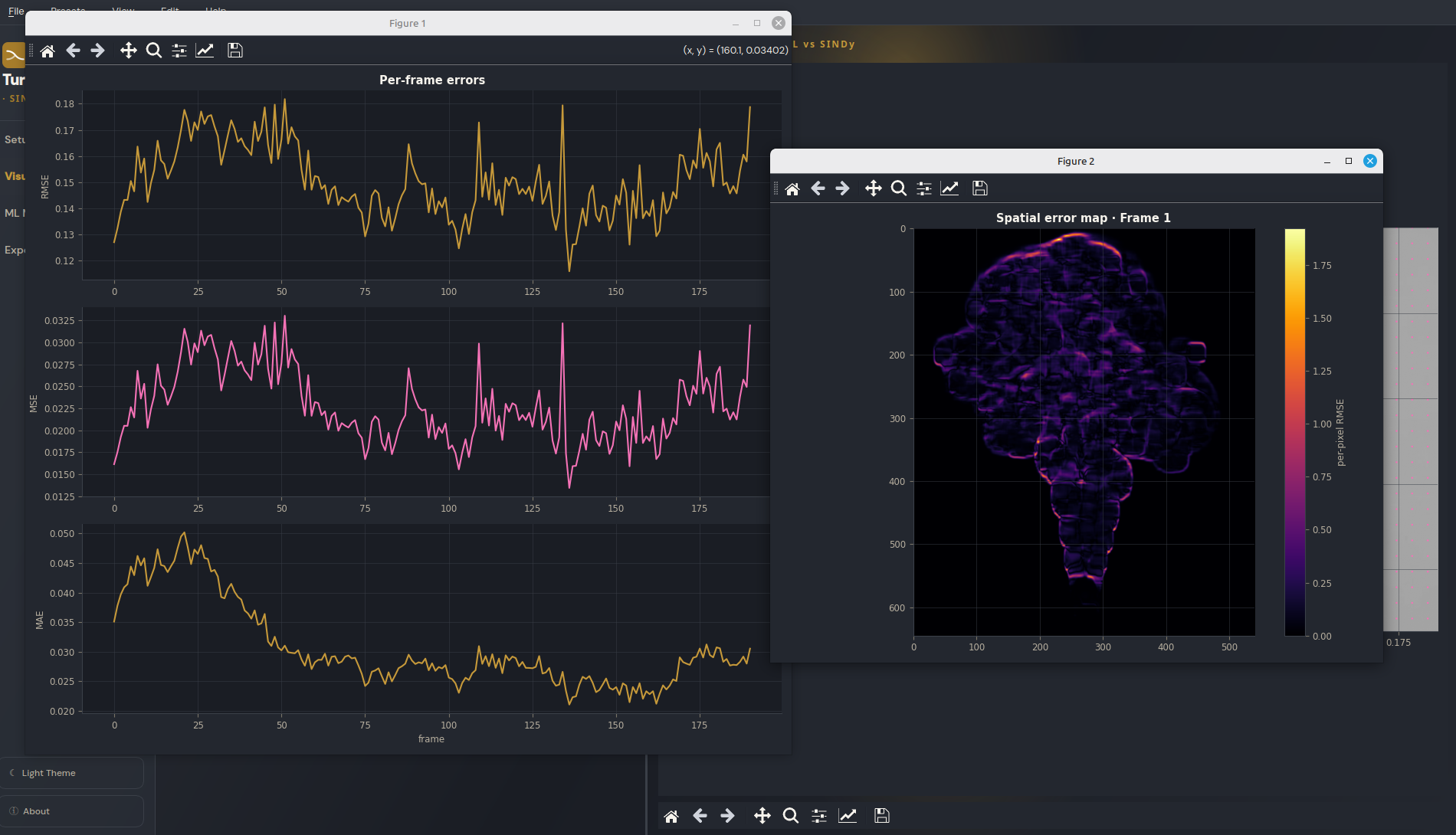
Validating a discovered equation used to be fragile. If one of the cross-validation folds hit a numerical edge case, the whole run stopped and you lost the rest of the results. The same was true when comparing different model settings.
Now each fold and each comparison run is isolated. A single failure is reported but does not stop the rest. You can compare libraries and settings confidently, knowing the results you see are real rather than the artifact of one bad fold.
A self-contained Windows installer
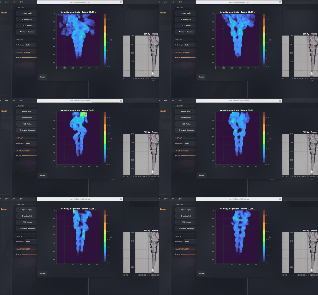
Earlier versions asked users to install PyTorch separately before machine-learning features would work. That broke the promise of a one-click installer. The new Windows installer now includes CPU-only PyTorch, the computer-vision library with all its extra modules, and the ONNX runtime, so everything works immediately after installation.
The installer is now 231 MB, but the trade-off is simple: open the file, accept the disclaimer, and start analyzing.
Tracker: from clicks to full physics reports
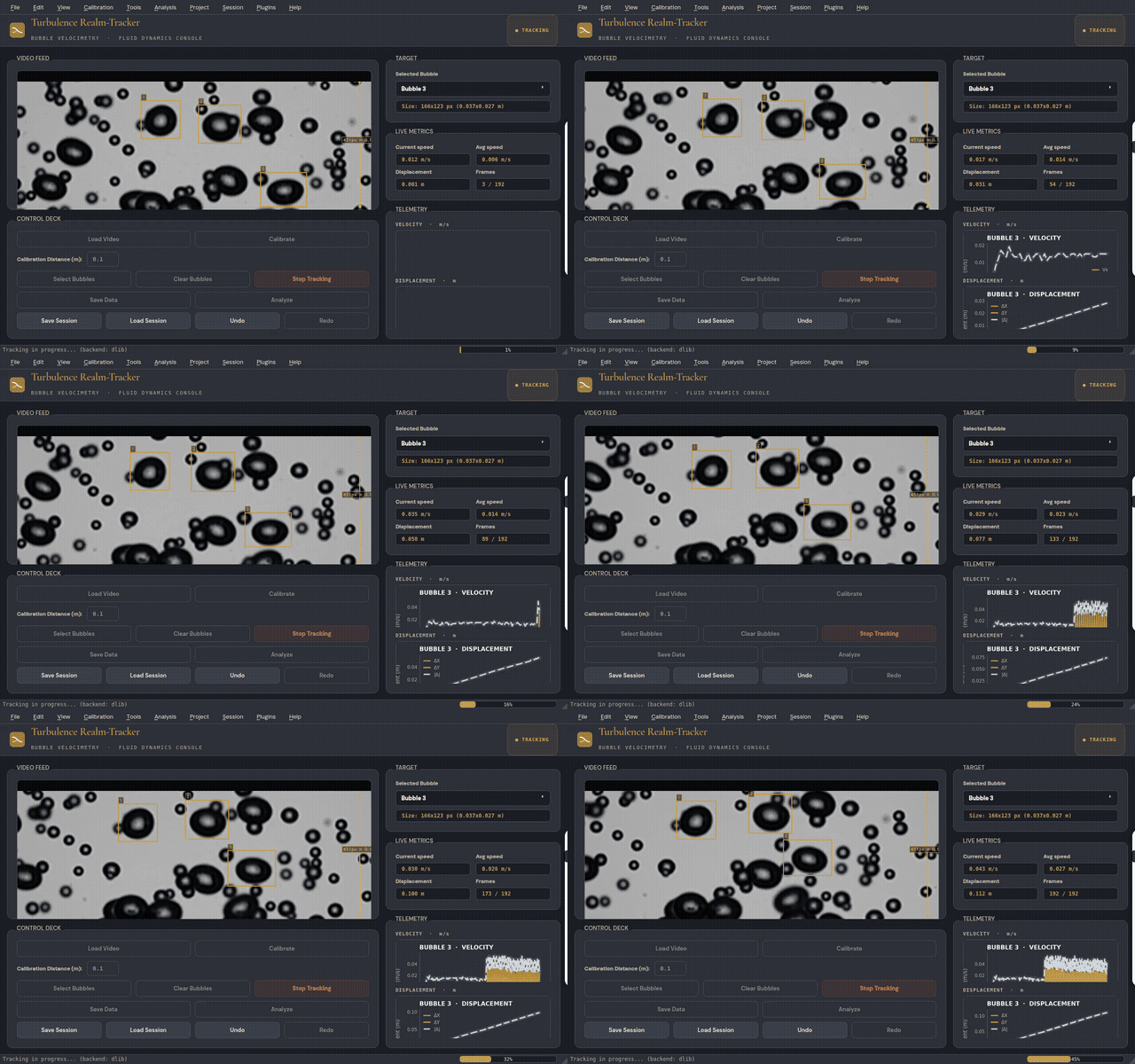
While SINDy was expanding its methods, Tracker was becoming a research instrument. Drop in a video of bubbles, droplets, or particles, and it will:
- Track every object automatically with multi-object tracking, so you do not have to click each bubble by hand.
- Segment bubbles even when they touch, and report size distributions, aspect ratios, and circularity.
- Compute fluid physics such as Reynolds, Weber, and Eötvös numbers, drag coefficients, and terminal-velocity comparisons with built-in presets for common fluids.
- Build Eulerian flow fields with dense optical-flow maps, speed contours, vorticity, and divergence.
- Detect events like coalescence, breakup, and detachment, and measure flux through a cross-section.
- Propagate uncertainty from calibration and localization into the reported speeds and error bars.
- Export a one-click PDF report with plots, tables, and statistics, plus a tidy table for notebooks.
AeroFlow NS: A 3D Navier-Stokes wind tunnel in your browser
While SINDy discovers equations from video and Tracker measures objects in video, AeroFlow NS goes the other direction: it generates the flow field from first principles, in real time, inside a web page. No install, no Python, no dependencies, just open an HTML file and orbit the camera.
The simulation builds two procedural aircraft from analytic signed distance fields, a refined jet airliner with winglets and engine nacelles, and a stealth flying-wing UCAV with a lambda planform and flat-shaded skin, and solves the incompressible Navier-Stokes equations on a 52×26×36 staggered MAC grid every frame. Semi-Lagrangian advection, pressure-Poisson projection, and immersed-boundary no-slip are all implemented in TypeScript. The wingtip vortices, wake, and stagnation point emerge from the solver, none are prescribed.
New capabilities in this release
Three controls have been added that make the simulation significantly more useful for exploration:
- GPU Tracers slider (500–10,000). Dial the particle count up or down in real time. The GPU buffer is allocated once at the maximum;
setDrawRangecontrols how many are simulated and drawn. No buffer reallocation when you move the slider. - Smoke flow visualization mode. A fourth visualization mode that renders particles as larger, softer, more opaque puffs, evoking the look of smoke or dye in a real wind tunnel. A
uSmokeuniform in the fragment shader widens the point size, softens the falloff, and increases opacity for a diffuse, continuous look. - Streamlines slider (10–200). Control the number of integrated streamlines. The upstream seed grid density scales proportionally, so you can go from a handful of diagnostic lines to a dense field of flow tracers.
Space freeze, G grid, O orbit.For a deep dive into the solver architecture, the staggered MAC grid, semi-Lagrangian advection, pressure-Poisson projection, immersed-boundary SDFs, and the GPU particle system, see the companion post: AeroFlow NS: A Real-Time 3D Navier-Stokes Wind Tunnel in Your Browser.
Download and try
Both desktop apps are available as signed installers for Windows and Linux. No Python installation is needed. Each installer displays a no-liability disclaimer that must be accepted before installation.
Download from turbulencerealm.com/download and follow the tutorials at turbulencerealm.com/tutorials.
AeroFlow NS requires no download at all, the two simulations embedded above are running right now in your browser. You can also open the airliner full-screen or open the stealth UCAV full-screen in a new tab.